Abstract. This paper presents our recent work on OMPS, a new timeline-based software architecture for planning and scheduling whose features support ...
A Multi-Component Framework for Planning and Scheduling Integration Amedeo Cesta, Simone Fratini and Federico Pecora ISTC-CNR, National Research Council of Italy Institute for Cognitive Science and Technology Rome, Italy {name.surname}@istc.cnr.it
Abstract This paper presents our recent work on O MPS, a new timeline-based software architecture for planning and scheduling whose features support software development for space mission planning applications. The architecture is based on the notions of domain components and is deeply grounded on constraint-based reasoning. Components are entities whose properties may vary in time and which model one or more physical subsystems which are relevant to a given planning context. Decisions can be taken on components, and constraints among decisions modify the components’ behaviors in time.
Introduction This paper describes O MPS, the Open Multi-component Planning and Scheduling architecture. O MPS implements a timeline-driven solving strategy. The choice of using timelines lies in their suitability for real-world problem specifications, particularly those of the space mission planning context. Furthermore, timelines are very close to the operational approach adopted by human planners in current space mission planning. Previous timeline-based approaches have been described in (Muscettola et al. 1992; Muscettola 1994; Cesta & Oddi 1996; Jonsson et al. 2000; Frank & J´onsson 2003; Smith, Frank, & Jonsson 2000). We are evolving from our previous work on a planner called O MP (Fratini & Cesta 2005) in which we have proposed a uniform view of state variables and resources timelines to integrate Planning & Scheduling (P&S). While the O MP experience lead to a proof of concept solver for small scale demonstration, the current development of O MPS is taking place within the Advanced Planning and Scheduling Initiative (APSI) of the European Space Agency (ESA). This has lead to a a substantial effort both in re-engineering and in extending our previous work. The general goal in O MPS is to provide a development environment for enabling the design and implementation of mission planning decision support systems to be used by ESA staff. O MPS also inherits our previous experience in developing planning and scheduling support tools for ESA, namely with the M EXAR, M EXAR 2 and R AXEM systems (Cesta et al. 2007), currently in active duty at ESA’s control center. Our aim within APSI is to generalize the approach to mission planning decision support by creating a
software framework that facilitates product development. The O MPS architecture is not only influenced by constraint-based reasoning work, but introduces also the notion of domain components as a primitive entity for knowledge modeling. Components are entities whose properties may vary in time and which model one or more physical subsystems which are relevant to a given planning context. Decisions can be taken on components, and constraints among decisions modify the components’ behaviors in time. Components provide the means to achieve modular decision support tool development. A component can be designed to incorporate into a constraint-based reasoning framework entire decisional modules which have been developed independently. The underlying philosophy of O MPS is to provide a development environment within which different, independently developed reasoning modules can be integrated seamlessly. It is useful to see a component as an entity having both static and dynamic aspects. Static descriptions are used to describe “what a component is”, e.g., the static property of a light bulb is that it can be “on” or “off”. Dynamic properties are instead those features which define how the static properties of the component may vary over time, e.g., a light bulb can go from “on” to “off” and vice-versa. It is tempting to associate components to the concept of state variable a la HSTS (Muscettola et al. 1992; Muscettola 1994). The reason for not doing so is that a state variable models an entity with static properties. The way this entity can change over time is typically specified through constraints on the possible transitions and durations of the states (e.g., through a timed automaton). A component as we define it here represents a more general concept: its behavior over time can be determined by non-trivial reasoning which is internal to the component itself. This distinction is important, as it provides a way to seamlessly incorporate into the O MPS reasoning framework objects which are themselves capable of modifying their behavior according to non-trivial processes, such as sophisticated reasoning algorithms. This paper is organized as follows. First, we define the basic building block, namely the component, providing examples which show how such an entity can be instantiated to represent a “classical” state variable, a resource, or even a more complex object whose temporal behavior can be described according to its own “internal dynamics”. Second, we describe the notion of decision on a component. Again,
we provide examples to show how this concept is instantiated on different common types of components. Third, we introduce the concepts of timeline and domain theory, the former providing the driving feature of the solving approach, the latter describing how components interact, and how decisions taken on components affects other components. Finally, we briefly illustrate the solving strategy implemented in the current O MPS framework and provide an example. It is worth saying that this paper describes the general approach underlying the O MPS architecture. We do not dwell on the theoretical aspects underlying the architecture, for which the interested reader is referred to (Fratini 2006).
Components and Behaviors An intrinsic property of components is that they evolve over time, and that decisions can be taken on components which alter their evolution. In O MPS, a component is an entity that has a set of possible temporal evolutions over an interval of time H. The component’s evolutions over time are named behaviors. Behaviors are modeled as temporal functions over H, and can be defined over continuous time or as stepwise constant functions of time. In general, a component can have many different behaviors. Each behavior describes a different way in which the component’s properties vary in time during the temporal interval of interest. It is in general possible to provide different representations for these behaviors, depending on (1) the chosen temporal model (continuous vs. discrete, or time point based vs. interval based), (2) the nature of the function’s range D (finite vs. infinite, continuous vs. discrete, symbolic vs. numeric) and (3) the type of function which describes a behavior (general, piecewise linear, piecewise constant, impulsive and so on). Not every function over a given temporal interval can be taken as a valid behavior for a component. The evolution of components in time is subject to “physical” constraints (or approximations thereof). We call consistent behaviors the ones that actually correspond to a possible evolution in time according to the real-world characteristics of the entity we are modeling. A component’s consistent behaviors are defined by means of consistency features. In essence, a consistency feature is a function f C which determines which behaviors adhere to physical attributes of the real-world entity modeled by the component. It is in general possible to have many different representations of a component’s consistency features: either explicit (e.g., tables or allowed bounds) or implicit (e.g., constraints, assertions, and so on). For instance, let us model a light bulb component. A light bulb’s behaviors can take three values: “on”, “off” and “burned”. Supposing the light bulb cannot be fixed, a rule could state that any behavior that takes the value “burned” at a time t is consistent if and only if such a value is taken also for any time t0 > t. This is a declarative approach to describing the consistency feature f C . Different actual representations for this function can be used, depending also on the representation of the behavior. A few more concrete examples of components and their associated consistency features are the following.
State variable. Behaviors: piecewise constant functions over a finite, discrete set of symbols which represent the values that can be taken by the state variable. Each behavior represents a different sequence of values taken by the component. Consistency Features: a set of sequence constraints, i.e., a set of rules that specify which transitions between allowed values are legal, and a set of lower and upper bounds on the duration of each allowed value. The model can be for instance represented as a timed automaton (Alur & Dill 1994) (e.g., the three state variables in Figure 2). Note that a distinguishing feature of a state variable is that not all the transitions between its values are allowed. Resource (renewable). Behaviors: integer or real functions of time, piecewise, linear, exponential or even more complex, depending on the model you want to set up. Each behavior represents a different profile of resource consumption. Consistency Feature: minimum and maximum availability. Each behavior is consistent if it lies between the minimum and maximum availability during the entire planning interval. Note that a distinguishing feature of a resource is that there are bounds of availability. In general, the component-based approach allows to accommodate a pre-existing solving component into a larger planning problem. For instance, it is possible to incorporate the M EXAR 2 application (Cesta et al. 2007) as a component, the consistency property of which is not computed directly on the values taken by the behaviors, but as a function of those behaviors1 .
Component Decisions Now that we have defined the concept of component as the fundamental building block of the O MPS architecture, the next step is to define how component behaviors can be altered (within the physical constraints imposed by consistency features). We define a component decision as a pair hτ, νi, where τ is a given temporal element, and ν is a value. Specifically, τ can be: • A time instant (TI) t representing a moment in time. • A time interval (TIN), a pair of TIs defining an interval [ts , te ) such that te > ts . The specific form of the value ν depends on the type of component on which the decision is defined. For instance, this can be an amount of resource usage for a resource component, or a disjunction of allowed values for a state variable. Regardless of the type of component, the value of any component decision can contain parameters. In O MPS, parameters can be numeric or enumerations, and can be used to express complex values, such as “transmit(?bitrate)” for a 1 Basically, it is computed as the difference between external uploads and the downloaded amount stated by the values taken by the behaviors. See (Cesta et al. 2007) for details on the M EXAR 2 application.
state variable which models a communications system. Further details on value parameters will be given in the following section.
Figure 1: The update function computes the results of a decision on a component’s set of behaviors. The figure exemplifies this effect given the two decisions: δ 0 imposes a value d0 for the behaviors of the component in the time instant t1 ; δ 00 imposes that the values of all behaviors converge to d00 after time instant t2 .
Overall, a component decision is something that happens somewhere in time and modifies a component’s behaviors as described by the value ν. In O MPS, the consequences of these decisions are computed by the components by means an update function f U . This is a function which determines how the component’s behaviors change as a consequence of a given decision. In other words, a decision changes a component’s set of behaviors, and f U describes how. A decision could state for instance “keep all the behaviors that are equal to d0 in t1 ” and another decision could state “all the behaviors must be equal to d00 after t2 ”. Given a decision on a component with a given set of behaviors, the update function computes the resulting set (see Figure 1). In the following, we instantiate the concept of decision for the two types of components we have introduced so far. State variable. Temporal element: a TIN. Value: a subset of values that can be taken by the state variable (the range of its behaviors) in the given time frame. Update Function: this kind of decision for a state variable implies the choice of values in a given time interval. In this case the subset of values are meant as a disjunction of allowed values in the given time interval. Applying a decision on a set of behaviors entails that all behaviors that do not take any of the chosen values in the given interval are excluded from the set. Resource (renewable). Temporal element: a TIN. Value: quantity of resource allocated in the given interval — a decision is basically an activity, an amount of allocated resource in a time interval. Update Function: the resource profile is modified by taking into account this allocation. Outside the specified interval the profile is not affected.
Domain Theory So far, we have defined components in isolation. When components are put together to model a real domain they cannot
be considered as reciprocally decoupled, rather we need to take into account the fact that they influence each other’s behavior. In O MPS, it is possible to specify such inter-component relations in what we call a domain theory. Specifically, given a set of components, a domain theory is a function f DT which defines how decisions taken on one component affect the behaviors of other components. Just as a consistency feature f C describes which behaviors are allowed with respect to the features of a single component, the domain theory specifies which of the behaviors belonging to all modeled components are concurrently admissible. In practice, a domain theory is a collection of synchronizations. A synchronization essentially represents a rule stating that a certain decision on a given component (called the reference component) can lead to the application of a new decision on another component (called target component). More specifically, a synchronization has the form hCi , V i −→ hCj , V 0 , Ri, where: Ci is the reference component; V is the value of a component decision on Ci which makes the synchronization applicable; Cj is the target component on which a new decision with value V 0 will be imposed; and R is a set of relations which bind the reference and target decisions. In order to clarify how such inter-component relationships are modeled as a domain theory, let us give an example. Example 1 The planning problem consists in deciding data transmission commands from a satellite orbiting Mars to Earth within given visibility windows. The spacecraft’s orbits for the entire mission are given, and are not subject to planning. The fundamental elements which constitute the system are: the satellite’s Transmission System (TS), which can be either in “transmit mode” on a given ground station or idle; the satellite’s Pointing System (PS); and the satellite’s battery (BAT). In addition, an external, uncontrollable set of properties is also given, namely Ground Station Visibility (GSV) and Solar Flux (SF). Station visibility windows are intervals of time in which given ground stations are available for transmission, while the solar flux represents the amount of power generated by the solar panels given the spacecraft’s orbit. since the orbits are given for the entire mission, the power provided by the solar flux is a given function of time sf(t). The satellite’s battery accumulates power through the solar flux and is discharged every time the satellite is slewing or transmitting data. Finally, it is required that the spacecraft’s battery is never discharged beyond a given minimum power level (in order to always maintain a minimum level of charge in case an emergency manoeuvre needs to be performed). Instantiation this example into the O MPS framework thus equates to defining five components: PS, TS and GSV. The spacecraft’s pointing and transmission systems, as well as station visibility are modeled with three state variables. The consistency features of these state variables (possible states, bounds on their duration, and allowed transitions) are depicted in Figure 2. The figure also shows the synchronizations involving the three components: one states that the value “locked(?st3)” on
Battery
Solar Flux sf(t)
power
power
max min time
time
cons(t)
Pointing System
?st1 != ?st2 ?st4 = ?st1
Unlocked(?st4) [1,+INF]
Transmission System Idle() [1+INF]
Slewing(?st1,?st2) [1,30]
?st2 = ?st3 ?st3 = ?st5
?st3 = ?st4
Locked(?st3) [1,+INF]
Transmit(?st5) [1,+INF]
?st3 = ?st6
Ground Station Visibility Visible(?st6) [1,+INF]
None() [1,+INF]
Figure 2: State variables and domain theory for the running example.
component PS requires the value “visible(?st6)” on component GSV (where ?st3 = ?st6, i.e., the two values must refer to the same station); another synchronization asserts that transmitting on a certain station requires the PS component to be locked on that station; lastly, both slewing and transmission entail the use of a constant amount of power from the battery. SF. The solar flux is modeled as a reusable resource. Given that the flight dynamics of the spacecraft are given (i.e., the angle of incidence of the Sun’s radiation with the solar panels is given), the profile of the solar flux resource is given function time sf(t) which is not subject to changes. Thus, decisions are never imposed on this component (i.e., the SF component has only one behavior), rather its behavior is solely responsible for determining power production on the battery (through the synchronization between the SF and BAT components). BAT. The spacecraft’s battery component is modeled as follows. Its consistency features are a maximum and minimum power level (max, min), the former representing the battery’s maximum capacity, the latter representing the battery’s minimum depth of discharge. The BAT component’s behavior is a temporal function bat(t) representing the battery’s level of charge. Assuming that power consumption decisions resulting from the TS and PS components are described by the function cons(t), the update function calculates the consequences of power production (sf(t)) and consumption on bat(t) as follows: Rt L0 + α 0 (sf(t) − cons(t))dt Rt if L0 + α 0 (sf(t) − cons(t))dt ≤ max; bat(t) = max otherwise. where L0 is the initial charge of the battery at the beginning of the planning horizon and α is a constant parameter which approximates the charging profile.
In summary, we employ components of three types: state variables to model the PS, TS and GSV elements, a reusable resource to maintain the solar flux profile, and an ad-hoc component to model the spacecraft’s battery. Notice that this latter component is essentially an extension of a reusable resource: whereas a reusable resource’s update function is trivially the sum operator (imposing an activity on a reusable resource entails that the resource’s availability is decreased by the value of the activity), the BAT’s update function calculates the consequences of activities as per the above integration over the planning horizon.
Decision Network The fundamental tool for defining dependencies among component decisions are relations, of which O MPS provides three types; temporal, value and parameter relations. Given two component decisions, a temporal relation is a constraint among the temporal elements of the two decisions. A temporal relation among two decisions A and B can prescribe temporal requirements such as those modeled by Allen’s interval algebra (Allen 1983), e.g., A EQUALS B, or A OVERLAPS [l,u] B. A value relation between two component decisions is a constraint among the values of the two decisions. A value relation among two decisions A and B can prescribe requirements such as A EQUALS B, or A DIFFERENT B (meaning that the value of decision A must be equal to or different from the value of decision B). Notice that temporal relations can involve any two component decisions, e.g., an activity (a resource decision) should occur BEFORE a value choice (a state variable decision). Conversely, value relations are defined among decisions pertaining to components of the same type. Lastly, a parameter relation among component decisions is a constraint among the values of the parameters of the two decisions. Such relations can prescribe linear inequalities between parameter variables. For instance, a parameter constraint between two decisions with values “available(?antenna, ?bandwidth)” and “transmit(?bitrate)” can be used to express the requirement that transmission should not use more than half the available bandwidth, i.e., ?bitrate ≤ 0.5·?bandwidth. Component decisions and relations are maintained in a decision network: given a set of components C, a decision network is a graph hV, Ei, where each vertex δC ∈ V is a component decisions defined on a component C ∈ C, and m n each edge (δC i , δC j ) is a temporal, value or parameter relam n tion among component decisions δC i and δC j . We now define the concepts of initial condition and goal. An initial condition for our problem consists in a set of value choices for the GSV state variable. These decisions reflect the visibility windows given by the Earth’s position with respect to the (given) orbit of the satellite. Notice that the allowed values of the GSV component are not references for a synchronization, thus they cannot lead to the insertion in the plan of new component decisions. Conversely, a goal consists in a set of component decisions which are intended to trigger the solving strategy to ex-
ploit the domain theory’s synchronizations to synthesize decisions. In our example, this set consists in value choices on the TS component which assert a desired number of “transmit(?st5)” values. Notice that these value choices can be allocated flexibly on the timeline. In general, the characterizing feature of decisions which define an initial condition is that these decisions do not lead to application of the domain theory. Conversely, goals directly or indirectly entail the need to apply synchronizations in order to reach domain theory compliance. This mechanism is the core of the solving process described in the following section.
mately represent a solution to the planning problem. Timeline management may introduce new component decisions as well as new relations to the decision network. For this reason, the O MPS solving process iterates domain theory application and timeline management steps until the decision network is fully justified and a consistent set of behaviors can be extracted from all component timelines. The specific procedures which compose timeline management are timeline extraction, timeline scheduling and timeline completion. Before showing how these procedures are composed to form the core of our planning approach, we describe the three steps in detail.
Reasoning About Timelines in O MPS
Timeline Extraction. The outcome of the domain theory application step is a decision network where all decisions are justified. Nevertheless, since every component decision’s temporal element (which can be a TI or TIN) is maintained in an underlying flexible temporal network, these decisions are not fixed in time, rather they are free to move between the temporal bounds obtained as a consequence of the temporal relations imposed on the temporal elements. For this reason, a timeline must be extracted from the decision network, i.e., the flexible placement of temporal elements implies the need of synthesizing a total ordering among floating decisions. Specifically, this process depends on the component for which extraction is performed. For a resource, for instance, the timeline is computed by ordering the allocated activities and summing the requirements of those that overlap. For a state variable, the effects of temporally overlapping decision are computed by intersecting the required values, to obtain (if possible) in each time interval a value which complies with all the decisions that overlap during the time interval.
O MPS implements a solving strategy which is based on the notion of timeline. A timeline is defined for a component as an ordered sequence of its values. A component’s timeline is defined by the set of decisions imposed on that component. Timelines represent the consequences of the component decisions over the time axis, i.e., a timeline for a component is the collection of all its behaviors as obtained by applying the f U function given the component decisions taken on it. The overall solving process implemented in O MPS is composed of three main steps, namely domain theory application, timeline management and solution extraction. More in detail, timeline management consists in extraction, scheduling and completion. Indeed, a fundamental principle of the O MPS approach is its timeline-driven solving process.
Domain Theory Application Component decisions possess an attribute which changes during the solving process, namely whether or not a decision is justified. O MPS’s domain application step consists in iteratively tagging decisions as justified according to the following rules (iterated over all decisions δ in the decision network): 1. If δ unifies with another decision in the network, then mark δ as justified;
Component decisions dur ∈ [30, 77]
A(x), B(y)
2. If δ’s value unifies with the reference value of a synchronization in the domain theory, then mark δ as justified and add the target decision(s) and relations to the decision network;
C(z)
3. If δ does not unify with any reference value in the domain theory, mark δ as justified.
⊥
The previous definition of initial condition and goal can be understood in terms of domain theory application as follows: an initial condition is a set of component decisions whose justification follows trivially from the domain, i.e., it is the direct result of the application of step 3; a goal, on the other hand, is a set of component decisions whose justification leads to the application of synchronizations in the domain theory (i.e., step 2).
Timeline Management Timeline management is a collection of procedures which are necessary to go from a set of decision network to a completely instantiated set of behaviors. These behaviors ulti-
[10, ∞)
dur ∈ [10, 23]
dur ∈ [20, 45]
B(y), C(z)
[30, ∞)
time
0
?
A(x), B(y) 10
30
B(y), C(z) 40
60
time
Timeline (EST)
Figure 3: Three value choices on a state variable, and the resulting earliest start time (EST) timeline.
In the current implementation, we follow for every type of component an earliest start-time (EST) approach, i.e., we have a timeline where all component decisions are assumed to occur at their earliest start time and last the shortest time possible. Figure 3 shows the timeline extraction mechanism for a state variable. The example illustrates two properties of timelines, namely flaws and inconsistencies. The first of these features depends on the fact that deci-
sions imposed on the state variable do not result in a complete coverage of the planning horizon with decisions. This timeline in the figure contains what we call a flaw in the interval [30, 40]. A flaw is a segment of time in which no decision has been taken, thus the state variable within this segment of time is not constrained to take on certain values, rather it can, in principle, assume any one of its allowed values. The process of deciding which value(s) are admissible with respect to the state variable’s internal consistency features (i.e., the component’s f C function) is clearly a nontrivial process. Indeed, this is precisely the objective of timeline completion. In addition to flaws, inconsistencies can arise in the timeline. The nature of inconsistencies depends on the specific component we are dealing with. In the case of state variables, an inconsistency occurs when two or more value choices whose intersection is empty overlap in time. In the example above, this occurs in the interval [0, 10]. As opposed to flaws, inconsistencies do not require the generation of additional component decisions, rather they can be resolved by posting further temporal constraints. For instance, the above inconsistency can be resolved by imposing a BEFORE constraint which forces (C(z)) to occur after (A(x), B(y)). In the case of the BAT component mentioned earlier, an inconsistency occurs when slewing and/or transmission decisions have lead to a situation in which bat(t) ≤ min for some t ∈ H. As in the previous example, BAT inconsistencies can be resolved by posting temporal constraints between the over-consuming activities. In general, we call the process of resolving inconsistencies timeline scheduling. Timeline Scheduling. The scheduling process deals with the problem of resolving inconsistencies. Once again, the process depends on the component. For a resource, activity overlapping results in an inconsistency if the combined usage of the overlapping activities requires more than the resource’s capacity. For a state variable, any overlapping of decision that requires a conflicting set of decisions must be avoided. The timeline scheduling process adds constraints to the decision network to avoid such inconsistencies through a constraint posting algorithm (Cesta, Oddi, & Smith 2002). Timeline Completion. This process is required for components such as state variables, where it is required that any interval of time in a solution is covered by a decision (this is trivially true for reusable resources as we have defined them in this paper). If it is not possible to force an ordering among decisions in such a way that entire planning horizon is decided, then a flaw completion routine is triggered. This step adds new decisions to the plan.
Solution Extraction Once domain application and timeline management have successfully converged on a set of timelines with no inconsistencies or flaws, the next step is to extract from the timelines one or more consistent behaviors. Recall that a behavior is one particular choice of values for each temporal segment in a component’s timeline. The previous domain theory application and timeline management steps have filtered
out all behaviors that are not, respectively, consistent with respect to the domain theory and the components’ consistency features. Behavior extraction deals with the problem of determining a consistent set of fully instantiated behaviors for every component. Since every segment of a timeline potentially represents a disjunction of values, behavior extraction must choose specific behaviors consistently. Furthermore, not all values in timeline segments are fully instantiated with respect to parameters, thus behavior extraction must also take into account the consistent instantiation of values across all components.
Overall Solving Process In the current O MPS solver the previously illustrated steps are interleaved as sketched in Figure 4.
Figure 4: The O MPS solving process. The first step in the planning process is domain theory application, whose aim is to support non-justified decisions. If there is no way to support all the decisions in the plan, the algorithm fails. Once every decision has been supported, the solver tries to extract a timeline for each component. At this point, it can happen that some timelines are not consistent, meaning that there exists a time interval over which conflicting decisions overlap (an inconsistency). In such a situation, a scheduling step is triggered. If the scheduler cannot solve all conflicts, the solver backtracks directly to domain theory application, and searches for a different way of supporting goals. If the solver manages to extract a conflict-free set of timelines, it then triggers a timeline-completion step on any timeline which is found to have flaws. It may happen that some timelines cannot be completed. In this case, the solver backtracks again to the previous domain theory application step, and again searches for a way of justifying all decisions. If the completion step succeeds for all timelines, the solver re-
turns to domain theory application, as timeline completion has added decisions which are not justified. Once all timelines are conflict-free and complete, the solver is ready to extract behaviors. If behavior extraction fails, the solver attempts to backtrack to timeline completion. This is because our currently implemented completion algorithm attempts to complete all incomplete timelines separately: thus it may easily happen that a completion over a timeline compromises behavior extraction on a different timeline (since values are linked with synchronizations). If this fails, the solver must return to domain theory application in order to search for a different plan altogether. Finally, the whole process ends when the solver succeeds in extracting at least one behavior for each timeline. This collection of mutually consistent behaviors represents a fully instantiated solution to the planning problem.
Figure 5: EST timelines for the TS and GSV state variables. Going back to our running example, the timelines of the GSV and TS components resulting from the application of a set of initial condition and goal decisions are shown in Figure 5 (no initial decision or goal is specified for the PS component). Notice that the GSV timeline is fully defined, reflecting the fact that the GSV component is not controllable, rather it represents the evolution in time of station visibility given the fully defined flight dynamics of the satellite. The TS timeline contains five “transmit” value choices, through which we represent our goal. These value choices are allocated within flexible time bounds (the figure shows an EST timeline for the component, in which these decisions are anchored to their earliest start time and duration). As opposed to the GSV timeline, the TS timeline contains flaws, and it is precisely these flaws that will be “filled” by the solving algorithm. In addition, the application during the solving process of the synchronization between the GSV and PS components that will determine the construction of the PS’s timeline (which is completely void of component decisions in the initial situation), reflecting the fact that it is necessary to point the satellite towards the visible target before initiating transmission. The behaviors extracted from the TS and PS components’ timelines after applying this solving procedure on our example are shown in Figure 6.
Related Work The synthesis of O MPS is aimed at creating an extensible problem solving architecture to support development of dif-
Figure 6: EST behaviors for the TS and PS state variables. ferent applications. It is worth making a comparison with other systems that, for different reasons, share the same goal with O MPS. Similarly to O MPS’s timelines, IxTeT (Ghallab & Laruelle 1994) follows a domain representation ontology based on state attributes which assume values in a given domain. Unlike O MPS in IxTeT system dynamics are represented with a STRIPS-like logical formalism. Resource reasoning is used as a conflict analyzer on top of the plan representation. Visopt ShopFloor (Bartak 2002) is grounded on the the idea of working with dynamic scheduling problems where it is not possible to describe in advance activity sets that have to be scheduled. That is the same principle behind the integration of planning into scheduling done in both O MP and O MPS: to put a domain theory behind a scheduling problem to gain flexibility in managing tasks and goal driven problem solving. Dynamic aspects of the problem are described using resources with complex behaviors. These resources are close to our state variable, but they are managed using global constraints instead of a precedence constraint posting approach as we are currently doing. Moreover, although we are working on P&S integration we maintain a clear distinction between planning and scheduling at the level of modeling problem features. HSTS (Muscettola et al. 1992; Muscettola 1994), has been the first to propose a modeling language with explicit representation of timelines, using the concept of state variables. In fact we are extending an HSTS-like state variables modeling language with a generic timeline oriented approach: in O MPS timelines represents not only state variable evolutions, but also multi-capacity and consumable resources, and may arrive to include generic components having temporal functions as behaviors. A clear difference w.r.t. HSTS is that in our approach we see different types of timelines as separate modules, while HSTS, and its derivatives RAX-PS and EUROPA, view resources as specialized state variables. Their view is certainly appealing but leaves the problem of integrating in a clean way multi-capacity resources open. In fact, while it is immediate to represent binary resources as state variables, it is quite difficult to model and handle cumulative resources. We believe that in these cases the best way is to exploit state of the art scheduling technologies hence our direction of seeing resources as an independent type of components.
Conclusions
Acknowledgments
In this article we have given a preliminary overview of O MPS a P&S system which follows a component-based, timeline-driven approach to planning and scheduling integration. The approach draws from and attempts to generalize our previous experience in mission planning tool development for ESA (Cesta et al. 2007) and to extend our previous work on the O MP planning system (Fratini & Cesta 2005). A distinctive feature of the O MPS architecture is that it provides a framework for reasoning about any entity which can be modeled as a component, i.e., as a set of properties that vary in time. This includes “classical” concepts such as state variables (as defined in HSTS (Muscettola et al. 1992; Muscettola 1994) and studied also in subsequent work (Cesta & Oddi 1996; Jonsson et al. 2000; Frank & J´onsson 2003)), and renewable/consumable resources (Laborie 2003; Cesta, Oddi, & Smith 2002). Another feature of the component-based architecture is the possibility to modularize the reasoning algorithms that are specific to each type of component within the component itself, e.g., profile-based scheduling routines for resource inconsistency resolution are implemented within the resource component itself. The more important consequence of this is the possibility to include previously implemented/deployed ad-hoc components within the framework. We have given an example of this in this paper with the battery component, which essentially extends a reusable resource. The ability to encapsulate potentially complex modules within O MPS components provides a strong added value in developing real-world planning systems. Specifically, this capability can be leveraged to include entire decisional modules which are already present in the overall decision process within which O MPS is deployed. An example is the M EXAR 2 system (Cesta et al. 2007)2 , whose ability to solve the Mars Express memory dumping problem can be encapsulated into an ad-hoc component. The ability to employ previously developed subsystems like M EXAR 2 benefits decision support system development in a number of ways. From the engineering point of view, it facilitates the task of fast prototyping, providing a means to incorporate complex functionality by employing previously developed decision support aids. Also, this feature contributes to increasing the reliability of development prototypes, as existing components (especially in the context of ESA mission planning) have typically undergone intensive testing before being deployed. Second, the componentbased architecture allows to leverage the efficiency of problem de-composition. Again, M EXAR 2 provides a meaningful example, as it is a highly optimized decision support system for solving the very specific problem of memory dumping. Lastly, the ability to re-use components brings with it the advantage of preserving potentially crucial user interface paradigms, the re-engineering of which may be a strong deterrent for adopting innovative problem solving strategies.
The Authors are currently supported by European Space Agency (ESA) within the Advanced Planning and Scheduling Initiative (APSI). APSI partners are VEGA GmbH, O N ERA , University of Milan and ISTC-CNR. Thanks to Angelo Oddi and Gabriella Cortellessa for their constant support, and to Carlo Matteo Scalzo for contributing an implementation of the battery component.
2
The M EXAR 2 system is a specific decision support aid developed by the Planning and Scheduling Team which is currently in daily use within ESA’s Mars Express mission.
References Allen, J. 1983. Maintaining knowledge about temporal intervals. Communications of the ACM 26(11):832–843. Alur, R., and Dill, D. L. 1994. A theory of timed automata. Theor. Comput. Sci. 126(2):183–235. Bartak, R. 2002. Visopt ShopFloor: On the edge of planning and scheduling. In van Hentenryck, P., ed., Proceedings of the 8th International Conference on Principles and Practice of Constraint Programming (CP2002), LNCS 2470, 587–602. Springer Verlag. Cesta, A., and Oddi, A. 1996. DDL.1: A Formal Description of a Constraint Representation Language for Physical Domains. In M.Ghallab, M., and Milani, A., eds., New Directions in AI Planning. IOS Press. Cesta, A.; Cortellessa, G.; Fratini, S.; Oddi, A.; and Policella, N. 2007. An innovative product for space mission planning – an a posteriori evaluation. In Proceedings of the 17th International Conference on Automated Planning & Scheduling (ICAPS-07). Cesta, A.; Oddi, A.; and Smith, S. F. 2002. A Constraint-based method for Project Scheduling with Time Windows. Journal of Heuristics 8(1):109–136. Frank, J., and J´onsson, A. 2003. Constraint-based attribute and interval planning. Constraints 8(4):339–364. Fratini, S., and Cesta, A. 2005. The Integration of Planning into Scheduling with OMP. In Proceedings of the 2nd Workshop on Integrating Planning into Scheduling (WIPIS) at AAAI-05, Pittsburgh, USA. Fratini, S. 2006. Integrating Planning and Scheduling in a Component-Based Perspective: from Theory to Practice. Ph.D. Dissertation, University of Rome “La Sapienza”, Faculty of Engineering, Department of Computer and System Science. Ghallab, M., and Laruelle, H. 1994. Representation and Control in IxTeT, a Temporal Planner. In Proceedings of the Second International Conference on Artifial Intelligence Planning Scheduling Systems. AAAI Press. Jonsson, A.; Morris, P.; Muscettola, N.; Rajan, K.; and Smith, B. 2000. Planning in Interplanetary Space: Theory and Practice. In Proceedings of the Fifth Int. Conf. on Artificial Intelligence Planning and Scheduling (AIPS-00). Laborie, P. 2003. Algorithms for Propagating Resource Constraints in AI Planning and Scheduling: Existing Approaches and new Results. Artificial Intelligence 143:151–188. Muscettola, N.; Smith, S.; Cesta, A.; and D’Aloisi, D. 1992. Coordinating Space Telescope Operations in an Integrated Planning and Scheduling Architecture. IEEE Control Systems 12(1):28–37. Muscettola, N. 1994. HSTS: Integrating Planning and Scheduling. In Zweben, M. and Fox, M.S., ed., Intelligent Scheduling. Morgan Kauffmann. Smith, D.; Frank, J.; and Jonsson, A. 2000. Bridging the gap between planning and scheduling. Knowledge Engineering Review 15(1):47–83.