A Multi-FPGA Application-Specific Architecture for Accelerating a Floating Point Fourier Integral Operator Jason Lee1, Lesley Shannon1, Matthew J. Yedlin2 and Gary F. Margrave3 1
Faculty of Applied Science Simon Fraser University {leeaj,lshannon}@sfu.ca
2
Department of Electrical and Computer Engineering University of British Columbia
[email protected]
Abstract
3
Department of Geoscience University of Calgary
[email protected]
Many complex systems require the use of floating point arithmetic that is exceedingly time consuming to perform on personal computers. However, floating point operators are also hardware resource intensive and require longer latencies than fixed point operators to complete. Due to the reduced logic density of FPGAs relative to ASICs, it is often only possible to accelerate a portion of a floating point application in hardware. This paper presents an application-specific architecture for the hardware acceleration of a complete Fourier Integral Operator (FIO) kernel used in seismic imaging on a multi-FPGA platform. The design utilizes several floating point computing elements (CEs) to calculate the FIO kernel in parallel stages on multiple FPGAs. A detailed study of floating point CEs, including a Fast Fourier Transform (FFT) CE, and a complete FIO prototype implementation on the BEE2 platform is described. The prototype implementation has a 12.4x increase in throughput over an optimized software implementation, and a predicted 15.8x increase in throughput on the BEE3 platform.
implemented on dedicated processors and GPUs. Furthermore, research has mainly focused on accelerating individual floating point operators [6][7][8] on FPGAs. This system exploits the inherent capabilities of hardware, using parallelism and pipelining to speed up the mathematical calculations. The final hardware implementation achieved a throughput speedup of 12.4x over an optimized software algorithm. Furthermore, synthesizing the design for the BEE3 platform resulted in a throughput speedup of 15.8x. The major contributions of this paper are: • An application-specific architecture to accelerate an FIO kernel, using scalable CE architectures • A detailed study of floating point FFTs • A prototype implementation on the BEE2 platform The remainder of this paper is structured as follows. Section 2 provides an overview of the FIO algorithm along with a background on available floating point FFT cores. The FIO system design is discussed in Section 3. Section 4 describes the floating point CE designs. Section 5 presents the performance results for individual CEs and the overall system. Finally, Section 6 concludes the paper along with providing suggestions for future work.
1. Introduction
2. Background
Field Programmable Gate Arrays (FPGAs) have been commonly used to accelerate fixed point DSP applications. Typically, floating point arithmetic was not used for these designs as it is extremely resource intensive [1]. Due to increasing resources available on modern FPGAs, floating point accelerators [2][3] are now being realized as Systemson-Chip [4] and full floating point applications are possible on multi-FPGA platforms. This paper presents a prototype hardware accelerated Fourier Integral Operator (FIO) kernel. The motivation for accelerating this application lies in its use in seismic imaging. Seismic imaging has many valuable applications, particularly for locating oil deposits using ultrasound like images of the earth. This application relies on the solution of complex mathematical equations that are exceedingly time consuming to execute on general purpose computers. A typical data sample set takes upwards of 20 days to process on a personal computer (PC). This application-specific architecture is developed for a multi-FPGA platform (BEE2)[5]. To the best knowledge of the authors, this application is the first multi-FPGA implementation of a complete floating point application. Typically, floating point applications have been
The following is a discussion of the implemented FIO algorithm. A summary of available FFT cores is also provided.
2.1 Seismic Imaging Application The purpose of seismic imaging is to obtain an extrapolated wavefield along a planar cross-section of the earth, taken from the surface, to produce an image of underground bodies. Figure 1 illustrates an example cross section.
Figure 1: Cross section of the earth Data is taken at multiple points along the earth’s surface, and the depth of a body determines the time it takes for a reflected wave to return to the same point. Our prototype employs a depth stepping method as described by Margrave et al [9]. The algorithm is divided into five major Computing Elements (CEs) for the
calculation of the single cross section shown in Figure 1. Figure 2 illustrates the data flow of the algorithm, highlighting these CEs.
architectures including fixed point and block floating point modes [14]. Due to resource requirements, Altera and Xilinx have targeted their FFT architectures towards their larger families of FPGAs. Since these commercial FFT cores were not freely available during the development our own FFT, this paper includes a study of the design costs and tradeoffs we investigated to create a scalable floating point FFT core.
3. Fourier Integral Operator Kernel in Seismic Imaging
Figure 2: FIO Data flow The function of each CE in the FIO kernel can be summarized as follows: CE1: Perform FFTs in the spatial domain CE2: Perform FFTs in the temporal domain CE3: Load segments of a pre-calculated phase matrix CE4: Perform a matrix multiplication on the transformed cross section CE5: Perform inverse FFTs back in to the spatial domain
Due to floating point resource requirements, the system is implemented as a multi-FPGA solution. The system is developed on the BEE2 platform [5], which is a general processing platform comprised of five Xilinx FPGAs (Virtex II Pro 70). Four of these FPGAs are configurable for user applications whereas the fifth FPGA acts as the platform controller. The BEE2 platform also provides 20GB of high speed, DDR2 DRAM memory. The five CEs are divided amongst the four user FPGAs. The single control FPGA is not used. The four user FPGAs are laid out in a ring topology with independent high speed parallel channels capable of transferring data at up to 10Gbps. Details on the development of an applicationspecific architecture and its implementation are given in the following section.
3.1 FIO System Design Figure 3 illustrates the FIO system block diagram partitioned into stages. How these stages are divided over FPGAs will be discussed in Section 5.4.
The phase matrix referred to in CE3 is generated by complex square roots and exponential operations, which are extremely resource intensive. Since this matrix is independent of the data, it can be pre-calculated in advance based on the appropriate velocity model and used repetitively for different sets of data. However, due to the size of the matrix, the entire matrix cannot be stored onchip and must be buffered from external memory in sections. The actual numerical processing occurs in CE4 when the extrapolated data vectors are multiplied with the buffered segments of the phase matrix.
2.2 Fast Fourier Transform To date Fast Fourier Transforms (FFTs) have largely been implemented in fixed point. Floating point FFTs have recently become commercially available. Dillon Engineering [10] now offers parameterized FFT cores that can be re-targeted towards specific FPGA and ASIC architectures. 4DSP [11] also offers a single precision floating point FFT implemented using a radix-32 or radix-2 butterfly architecture. These cores are targeted at both Xilinx and Altera devices. Previous research has also investigated double-precision floating point FFTs on FPGAs [12]. Altera and Xilinx both offer block floating point FFT. Block floating point is a compromise between fixed point performance and floating point dynamic range. It allows floating point calculations to be performed on fixed point hardware by shifting the data to share a common exponent for a block of data The Altera FFT [13] core implements a radix-2/4 decimation-in-frequency (DIF) FFT algorithm for transform lengths of 64 to 4k points. In its LogiCore package, Xilinx’s FFT provides four different FFT
Figure 3: Block diagram of FIO system Figure 3 illustrates the flow of data between CEs in the multi-FPGA platform. The architecture consists of three stages. Stage 1 transforms the data in the spatial domain using CE1. Stage 2 includes CE2, CE3, and CE4. This stage takes the transformed data, performs a temporal FFT, and processes it by performing a matrix multiply. Finally, Stage 3 uses CE5 to perform an inverse spatial FFT.
A set of data constitutes 1024 surface sample points (columns) in the spatial domain (the earth’s surface) with 256 data samples (rows) of varying time (depth) at each surface point. Initially, the data set is transformed in the spatial domain, row by row, for all time (depth) measurements via a 1024-point FFT (CE1). The FFT must be performed on all the rows of the entire matrix before the next stage can begin processing. The initial data is loaded from Memory A to the FFT. As each row is completed the resultant is transferred to Stage 2 and stored in Memory B. When the last 1024-point FFT is completed, the first stage is finished and the second stage can initiate while Stage 1 begins processing a new data set. Stage 3, which consists of CE5, mirrors Stage 1 in operation. It performs an inverse FFT along each row in the same fashion once a complete data set has been processed in Stage 2. When Stage 2 initiates, CE2 performs a 256-point FFT along each column of data. As each column is completed, the resultant is transferred to CE4 for the matrix multiply in order to allow CE2 to continue processing temporal FFTs in parallel. CE4 takes the 256 points and multiplies it with the buffered 256x256 phase matrix loaded from Memory C by CE3. The resultant is then transferred to Stage 3 and stored in Memory D. Each stage has a single MicroBlaze (soft processor core) that receives data from the previous stage to store in external memory. When the previous stage runs to completion, this MicroBlaze is then used to load the stored data for processing in its respective stage. Since the system is split into three stages, the system can act as a three stage pipeline, processing three sets of data in parallel. In order to facilitate inter-CE communication, the Systems Integrating Modules with Predefined Physical Links (SIMPPL) model for application specific architectures is used [15]. SIMPPL is an architectural model that facilitates rapid integration of modules for SoC designs by using fixed communication protocols and physical links to facilitate system integration. This allows designers to focus on their CE designs for their applicationspecific architectures. Originally intended for on-chip communication in SoCs, this framework has been extended to multi-chip platforms [16]. The extended protocol abstracts inter-FPGA communication such that the multiFPGA platform resembles a single large reconfigurable platform.
4. Hardware Accelerated Floating Point Operators Implementing floating point arithmetic applications on an FPGA is challenging since basic operations require significant resources. Table 1 shows some of the resource requirements for performing complex single precision floating point operations and complex 32-bit fixed point operations obtained from Xilinx data sheets [17][18][19]. Table 1: Arithmetic operation resource usage Floating Point Fixed Point Operation FFs LUTs FFs LUTs Add 1 182 1 160 116 106 Subtract 1 182 1 160 116 106 Multiply* 1 732 1 530 170 154 *Includes the use of embedded multipliers. Based on these results, the complexity of computing elements is limited by the resources available on an FPGA. For example, an FPGA with 100,000 Flip-Flops (FFs) could only implement 57 complex floating point multipliers. The following sections describe the design of the floating point computing elements.
4.1 Fast Fourier Transform A common method of performing an FFT is the Cooley-Tukey algorithm [20]. Many available FFT cores employ this algorithm including Xilinx’s FFT. This algorithm partitions the transform into smaller operations called butterflies. A radix-2 decimation-in-time (DIT) butterfly is used in the design. Figure 4 illustrates how a single butterfly is implemented for our system.
Figure 4: Single butterfly Each butterfly performs an operation on two points of data, multiplying one by a twiddle factor and subsequently adding and subtracting these values from the initial points of data. A table of twiddle factors and butterflies are used to compute the complete FFT. For example, to achieve the highest throughput for an 8-point FFT, it should be pipelined into three stages of butterflies, as shown in Figure 5.
Figure 5: 8 point FFT The seismic imaging application requires two FFTs of at least 1024 and 256-points. The primary concern when developing these FFTs was the amount of resources they require. One butterfly requires a floating point multiply, subtract and add, which totals approximately 4,000 FFs based on resource usages in Table 1. As an FFT increases in size, the number of butterflies and resource requirements scale at a log-linear rate. For example, a 256-point FFT requires 8 stages of 128 butterflies. This totals over 4 million FFs, which exceeds the resources on all available commercial FPGAs. In order to implement a large FFT on a smaller FPGA, the CE is designed to use a fixed bank of butterflies. This is beneficial since the FFT CE can be scaled according to available resources. Figure 6 shows the designed architecture for the FFTs (CE1, CE2, and CE5).
4.3 Phase Matrix Buffer As previously described in Section 2.1, the phase matrix is pre-calculated before runtime and loaded into the system. Figure 8 shows the design used to buffer the matrix into the system in CE3.
Loader
BRAM
Unloader
Figure 6: FFT block diagram Similar to Stage 1 of the FFT shown in Figure 5, the butterfly bank contains an array of butterflies. While throughput is decreased in comparison to the fully pipelined FFT given in Figure 5, a fixed butterfly bank makes large FFTs possible. The input data is initially transferred into the FFT and is loaded into the single bank of butterflies by the loader to perform each stage incrementally. The unloader takes the result and loops the data back to the memory block. The loader then repeats the process for a given number of iterations. For example, a 1024-point FFT normally requires 4608 butterflies. If the butterfly bank contains 8 butterflies, the data would loop through the bank 576 times. The optimal butterfly bank size from our investigation is discussed in Section 5.1.
4.2 Complex Matrix Multipliers The Complex Matrix Multiply (CMM) is used to process the data in CE4. Figure 7 illustrates the architecture that was designed.
BRAM
Figure 8: Block diagram of PMG The designed CE consists of multiple memory blocks, which are loaded in parallel. A single memory block contains a set of 256 points which is unloaded sequentially into the CMM as it is needed. The optimal number of memory blocks, and how they are loaded is found in Section 5.3.
5. Results A timing analysis of each CE was performed in order to determine the optimal design. The following sections give the results for each CE, as well as the final results for the complete FIO kernel.
5.1 Fast Fourier Transform In order to determine the number of banks to be used in the FFT CEs, the tradeoffs between the number of banks and speedup was determined. Table 2 gives the latency and resource requirements for a 1024-point FFT using a varying number of butterflies. Table 2: Latency for varying butterfly banks
# of Butterflies 1 2 4 8 16
Figure 7: Complex matrix multiply block diagram The CMM contains two shift registers, a stage of multipliers, multiple stages of adders, and an accumulation stage. The number of adder stages depends on how many data points are calculated at a given time. Determining the optimal number of data points used for a CMM is presented in Section 5.2. The purpose of the CE is to take a column of data produced by the 256-point FFT and multiply it by a 256x256 phase matrix. The CMM multiplies a segment of the 256-point temporal FFT vector by a segment of the phase matrix and accumulates the results. The final accumulation stage sums the results over the number of temporal data points (e.g. 256). For example, if a 256x256 multiply needs to be performed, and the core calculates 8x8 points at a time, the core iterates 32 times and the accumulation stage adds the total from each iteration to output the final result.
Latency (cycles) 107 520 53 760 30 720 29 540 27 310
Area (FFs) 6 042 11 376 20 387 38 479 75 192
Area (LUTs) 6 038 10 085 18 170 34 340 66 680
Based on the results, speedup is roughly doubled whenever the number of butterflies is doubled from one to four butterflies. However, when moving from four to eight butterflies speedup is only increased 1.04x while area is increased by 1.89x. This is due to different pipeline operation latencies in the design. In order to optimize the FFT design, each operation in the computation should have equal latencies. The longest fixed latency is the floating point multiplier supplied by Xilinx. This operation requires 21 clock cycles. For our load sequence, loading data for four butterflies take 24 clock cycles. Using more or less than four butterflies would increase the discrepancy in latency between the load and the multiplier. Therefore, we chose to use four butterflies in our fixed butterfly bank. Using this design, Table 3 lists the latencies of varying FFT lengths on different FPGAs using a fixed butterfly bank of four.
n-Point FFT 128 256 512 1 024 2 048 4 096
Table 3: FFT latency Latency (microseconds) V2Pro V4 12.39 10.75 28.31 24.58 63.71 55.29 141.56 122.88 311.44 270.34 679.52 589.82
V5
2048 clock cycles to unload four memory blocks sequentially into the CMM. These results in balanced load and unload latencies. 9.77 22.34 50.27 111.71 245.76 536.20
Since the same design is used for varying FFT lengths, the resource requirements are the same for all lengths. In order to increase throughput, the FFT must be further pipelined or a faster multiplier needs to be used. Other options that were explored included using parallel banks of butterflies within a single FFT CE shown in Figure 6 or using multiple copies of FFT CEs in parallel. Table 4 compares the latency and throughput for these two options for a 1024point FFT. Throughput is calculated based on data sets/100,000cycles.
# Parallel Latency Throughput
Table 4: Parallel FFT latency Parallel Banks Parallel FFT CEs 2
4
8
2
4
8
4.15
5.83
7.30
5.28
10.58
21.1
24064
17152
13696
37888
37888
37888
Throughput increases faster for parallel FFT CEs since multiple FFTs on different data sets can be calculated concurrently, as opposed to reducing the number of iterations to calculate a single data set. Therefore, based on the results, it was determined that it was more beneficial to use multiple FFT CEs rather than using multiple fixed butterfly banks within an FFT CE. In comparison to other commercially available floating point FFTs, such as 4DSP [11], our FFT has longer processing latencies. However, it was determined that the bottleneck in our system is the CMM and optimizing the FFT was not the main focus. Our objective was to optimize the complete floating point application.
5.2 Complex Matrix Multiply For an optimal design, the pipeline operations in the CMM must be approximately the same. Similar to the FFT CE, the bottleneck was the Xilinx floating point multiplier. Therefore, each stage is designed to have a latency of approximately 21 clock cycles. For each matrix multiply iteration, a complex single precision number takes 2 clock cycles to load. Therefore, the design operates on eight data points for a load time of 16 clock cycles. A 16x16 multiply would result in significant area increase and a load stage of 32 clock cycles, which is longer than the multiplier operation. Therefore, the design consists of one stage of four multipliers, three adder stages, and a final accumulation stage. The latency to calculate a 256x256 multiply is 771 clock cycles, and the latency to compute the complete data set (256*256x256) is 172 115 clock cycles.
5.3 Phase Matrix Buffer The phase matrix buffer (PMB) needs to be capable of supplying the CMM with a new set of 256 points every 512 clock cycles. One memory block takes 2048 clock cycles to load. Thus, eight memory blocks are used in the design. Four memory blocks are loaded in parallel while the other four are unloaded into the CMM. Therefore, it takes 2048 clock cycles to load four memory blocks in parallel and
5.4 Fourier Integral Operator Using the described CEs, the latencies of each CE is measured for the BEE2 platform. These results include the calculated latencies to transmit the data between FPGAs over onboard LVC-MOS parallel trace connections [14]. Table 5 gives the latency results and resource requirements for each module in the system, running at a max frequency of 195MHz. Currently, the max frequency is limited by the MicroBlaze. Module 1024-FFT 256-FFT CMM PMB 1024-IFFT
Table 5: CE latency
Area FFs LUTs 20 387 18 170 20 387 18 170 26 643 24 672 1 638 1 549 20 387 18 170
Latency
Runtime (us)
37 888 7 936 172 115 2 048 37 888
194.29 40.69 882.64 105.02 194.29
Based on these results, it was determined that inter-FPGA communication is not a bottleneck in the system as the CE latencies are orders of magnitude greater than the data transfer latencies. However, external memory access is a bottleneck in some parts of the design particularly the CMM (CE4) and PMB (CE3). A more sophisticated DRAM scheduler will result in speedups in throughput and latency by increasing max frequency and decreasing load latencies. In order to speedup throughput, multiple CEs are used in parallel. From the results in Table 5, the CMM has the longest latency. Therefore, to significantly increase throughput, multiple CMMs are performed in parallel. Based on available resources on the BEE2 platform, 2CE1s, 1-CE2, 2-CE3s, and 2-CE4s are used. 1 CMM requires 4 banks of memory and approximately 35,000 FFs. Since each FPGA on the BEE2 platform offers four banks of memory, two FPGAs are dedicated to perform the CMMs. The CEs from the block diagram in Figure 3 are divided over FPGAs as follows: • • • •
FPGA 1: 2-CE1, 1-CE2 FPGA 2: 1-CE3, 1-CE4 FPGA 3: 1-CE3, 1-CE4 FPGA 4: 1-CE5
Table 6 lists the total latency for each stage of the system based on this FPGA partitioning. The latencies of each stage include the inter-FPGA communication latencies. Throughput is given in data sets/100 seconds, and runtime in microseconds given the running max frequency of 195MHz. Module Stage 1 Stage 2 Stage 3
Table 6: Total latency of stages Area FFs 41 901 80 524 41 901
Latency
LUTs 39 732 75 299 39 259
9 699 328 88 302 931 9 699 328
Runtime (us) 0.04974 0.45283 0.04974
The total latency of the system is measured and compared with the equivalent vector optimized Matlab algorithm run in single precision floating point. Initial work on a C-code implementation of the algorithm was also generated. However, the original unoptimized version was
approximately four times slower than the optimized Matlab code. As optimizing the C code would only result in up to an additional two times speedup over the optimized Matlab code, it was decided that focusing on the development of the hardware implementation would be more constructive, resulting in significantly more speed up. The software algorithm is run on a PC with a 2.13GHz Intel Core 2 Duo and 4GB of RAM. Table 7 shows the speedup for our prototype application specific architecture. Latency is measured in seconds, and throughput in data sets/100 seconds. Table 7: Speedup of HW prototype application Hardware Matlab Speedup Platform BEE21 (195MHz) Latency 0.55231 5.621 10.17 Throughput 220.611 17.79 12.39 BEE3 (248MHz) Latency 0.43428 5.621 12.94 Throughput 280.632 17.79 15.77 The prototype implementation on the BEE2 platform results in throughput speedup of 12.4x. With more FPGA resources and faster chips, a further increase in speedup is achievable as indicated in the BEE3 results. Currently, the max frequency for both platforms is limited by the MicroBlaze. Therefore, significant speedup can also be attained by replacing the MicroBlaze with a more sophisticated DRAM scheduler.
Acknowledgements We acknowledge Xilinx and CMC Microsystems for providing the tools, development hardware and computing equipment. Thanks to NSERC for funding provided to Lesley Shannon.
8. References [1]
[2]
[3]
[4] [5] [6]
[7]
6. Conclusions and Future Work This paper presents the prototype for an applicationspecific architecture of an FIO kernel. As part of the design process, a detailed study on floating point CEs, particularly the FFT CE, was performed. This resulted in configurable CEs that are scalable for different FPGA devices. The system runs on the BEE2 platform achieving a throughput speedup of 12.4x over an optimized software implementation. The prototype was also scaled and resynthesized for the BEE3 platform, which has the newer Virtex 5 FPGAs, for a predicted throughput speedup of 15.8x. While our FFT is slower than the Xilinx block floating point FFT, this is not the bottleneck. External memory access and the use of MicroBlazes to manage memory access is the current performance bottleneck in the prototype implantation. Future work includes implementing more sophisticated dedicated DRAM scheduling for memory access. This will reduce memory access times and therefore the latency of the FIO CEs. Furthermore, significant resource usage and latency is incurred due to the normalization and denormalization of floating point numbers. We will also investigate internal representations of floating point input data within the FIO kernel that reduce or limit these operations, such as block floating point, to further decrease latency. However, it will be necessary to verify that the required computational precision is maintained before these representations can be employed.
[8]
[9]
[10] [11] [12]
[13] [14] [15]
[16]
[17] [18] [19] [20]
1
The individual CEs have been mapped onto the BEE2 platform and have been verified to run in hardware using the Xilinx XUPV2Pro development board [21] and the Xilinx ML505 development board [22]. However, there have been problems loading the final design onto the actual BEE2 platform. Total latency measurements found in Table 6 include a worst case latency measurement for inter-FPGA communication.
[21] [22]
W.B. Ligon, S. McMillan, G. Monn, K. Schoonover, F. Stivers, K.D. Underwood, “A re-evaluation of the practicality of floating point operations on FPGAs,” In Proceedings of the IEEE Symposium on FPGAs for Custom Computing Machines, April 1998, pp. 206-215. K.D. Underwood, K.S. Hemmert, “Closing the Gap: CPU and FPGA trends in Sustainable Floating-Point BLAS Performance,” In Proceedings of the IEEE Symposium of Field Programmable Custom Computing Machines, 2004, pp. 219-228. G.R. Morris, V,K. Prasanna, “An FPGA-Based FloatingPoint Jacobi Iterative Solver,” In Proceedings of the 8th International Symposium on Parallel Architectures, Algorithms and Networks, 2005, pp. 420-427. J. Greenbaum, “Reconfigurable Logic in SoC Systems, “ In Proceedings of the IEEE Custom Integrated Circuits Conference, 2002, pp. 5-8. C. Chang, J. Wawrzynek, and R.W. Brodersen, “BEE2: A High-End Reconfigurable Computing System,” IEEE Design & Test of Computers, April 2005, pp 114-125. N. Shirazi, A. Walters, P. Athanas, “Quantitative analysis of floating point arithmetic on FPGA based custom computing machines.” InProceedings of the IEEE Symposium on FPGA’s for Custom Computing Machines, p. 155, 1995. J. Detrey, F. Dinechin, “Parameterized floating-point logarithm and exponential functions for FPGAs,” Microprocessors and Microsystems, Vo. 31, Issue 8, pp 537-545, 2007. G. Morris, “Floating-Point Computations on reconfigurable Computers,” In Proceedings of the 2007 DoD High Performance Computing Modernization Program Users Group Conference, pp. 339-344, 2007. G.F. Margrave, H.D. Geiger, S.M. Al-Saleh, and M.P. Lamoureux, “Improving explicit seismic depth migration with a stabilizing Wiener filter and spatial resampling,” Geophysics, Vol. 71, No. 3, 2006, pp. S111-S120 Dillon Engineering, Inc. “Ultra High-Performance FFT/IFFT IP Core,” 2007. 4DSP, “Floating Point Fast Fourier Transform,” September 2007. K.S. Hemmert, K.D. Underwood, “An Analysis of the Double-Precision Floating-Point FFT on FPGAs,” In Proceedings of the 13th Annual IEEE Symposium on Field Programmable Custom Computing Machines, pp. 171-180, 2005. Altera, “FFT MegaCore Function User Guide,” MegaCore Version 7.0, October 2007. Xilinx, “Fast Fourier Transform v5.0,” October 10, 2007. L. Shannon, Paul Chow, “SIMPPL: An Adaptable SoC Framework using a Programmable Controller IP Interface to Facilitate Design Reuse,” IEEE Transactions on VLSI Systems, Vol 15, Issue 4, pp 377-390, April 2007. D. Dickin, L.Shannon, “Extending the SIMPPL SoC Architectural Framework to Support Application-Specific Architectures on Multi-FPGA Platforms,” Proceedings of the 19th Annual IEEE Symposium on Application-specific Systems, Architectures, and Processors, July 2008. Xilinx, “Multiplier v10.0,” April 2, 2007. Xilinx, “Floating Point Operator v3.0,” September 29. 2006. Xilinx, “Adder/Subtractor v7.0,” December 11, 2003. J.W. Cooley, and J. Tukey, “An Algorithm for the Machine Calculation of Complex Fourier Series,” Mathematics of Computation, Vol. 19, No. 90, April 1965, pp. 297-391. Xilinx, “Xilinx University Program Virtex-II Pro Development System,” March 8, 2005. Xilinx, “ML505/ML506 Evaluation Platform,” October 30, 2007.