A Multi-Objective Programming Model for Disaster Preparedness ...

International Journal of Applied Operational Research Vol. 5, No. 3, pp. 41-57, Summer 2015 Journal homepage: ijorlu.liau.ac.ir

A Multi-Objective Programming Model for Disaster Preparedness Planning M. Rabbani*, A. Farshbaf Geranmayeh, N. Manavizadeh

Received: 29 October 2014 ;

Accepted: 4 April 2015

Abstract Nowadays, the necessity of accurate quantitative decision support methods is becoming a critical subject for managers as rivalry between organizations caused a more fragile economic environment and brand reputation is becoming more important. Furthermore, dealing with incidents after they happened is not accepted by customers anymore. Managers require powerful decision making tools to support them in handling crisis situations, and also protecting their brand reputation and image of their organization. In this paper a new multi-objective programing model for disaster preparedness planning problem has been developed to deal with the negative impacts of a specific disaster on the organization’s key functions with uncertain properties. Finally, a heuristic sensitivity analysis approach is proposed in order to validate the results. Keywords: Disaster Recovery Planning (DRP), Disaster Preparedness Planning (DPP), Multi-Objective Programing (MOP), Highest Effectiveness Approach (HEA).

1 Introduction Robust continuity of the organizations after catastrophic events highly depends on their preparedness planning that they have done. In today’s delicate economic environment, business owners realize the importance of ensuring organization preparedness against catastrophic events that might have a disastrous impact on their financial well-being [1]. For business owners, preparedness means staying in business after a disaster. Natural disasters (such as earthquakes, hurricanes and floods) and man-made mistakes (such as fire, explosion) are just some examples of major disasters that can lead to widespread disruptions and failure of organizations [2, 3]. Over the past 30 years, various factors including the increasing occurrence of disastrous events and government regulations in some industries have resulted in intense interest in the development of disaster recovery planning and strategies (DRP/S). DRP is the continuous * Corresponding Author. () E-mail: [email protected] (M. Rabbani) M. Rabbani Professor, Department of Industrial Engineering, College of Engineering, University of Tehran, Tehran, Iran A. Farshbaf-Geranmayeh Ph.D. Candidate, Department of Industrial Engineering, College of Engineering, University of Tehran, Tehran, Iran N. Manavizadeh Assistant Professor, Department of Industrial Engineering, KHATAM Institute of Higher Education, Tehran, Iran

42

M. Rabbani, et al. / IJAOR Vol. 5, No. 3, 41-57, Summer 2015 (Serial #17)

process of preparing for quick recovery of critical processes and infrastructures of an organization. A good DRP can help businesses devise plans for recovering from business interruption, financial losses and also help them to protect their employees, the community and the environment. Disaster recovery plans usually aims at minimizing potential loss by systematic identification, assessment, prioritization of risks that are inconvenient to business functions [4] and protecting key business functions and assets that need the most protection by providing strategies that ensure a complete restoration of key functions considering resource limitations within a tolerable time when a disruption occurs. The methodology for implementing a DRP consists of five phases [2]: Identifying potential risks and conducting a risk assessment (RA), performing a business impact analysis (BIA), developing recovery strategies, publishing the plan, disseminating it to employees and training them, and finally examining the plan, testing through a real-life situation and correcting plan deficiencies.

1.1 Motivation and significance Although DRP has become increasingly an interesting subject for managers and business leaders, there have been few studies consisting mathematical formulation in this area, particularly when it comes to increase the recovery capabilities of organizations with an efficient and economic manner. Natural disasters have potentially severe economic consequences in terms of properties damage and business interruptions. Previous studies have neglected to consider the economic aspects of disaster preparedness planning quantitatively in optimization models. Accordingly, the contribution of this paper is developing a model that ensures the preparedness of the organization for complete economic recovery with an acceptable reliability throughout a specific time horizon when the occurrence of a single disaster is anticipated. In this paper, a new Mixed-Integer Non-Linear Programming (MINLP) model has been presented that optimizes the cash flow spending on resources during the planning horizon in order to minimize costs and maximize the reliability simultaneously by considering time and resource limitations. Moreover, the Highest Effectiveness Approach (HEA) is developed to deal with uncertainty, analyze obtained results, and validate the proposed model. The remainder of the paper is organized as follows: Section 2 provides a review of disaster recovery problems followed by economic study of disasters. In Section 3 a mixedinteger non-linear programming model for disaster preparedness planning (DPP) problem is developed. Section 4 presents a solution methodology for multi-objective model which is followed by a heuristic approach to deal with uncertainty. In section 5 a numerical example is illustrated and the test problem is validated by performing sensitivity analysis. Finally, Section 6 presents conclusions and suggestions for further research.

2 Literature review For the first time, [5] classified all the potential disasters into a finite number of categories in order to gain maximum information about all possible accidents without demanding an excessive budget such that the impact of all accidents in each category would be approximately identical. From this a measure of similarity is defined between each category, so it is possible to have an estimation of damage and occurrence probability for each category.

A Multi-Objective Programming Model for Disaster Preparedness Planning

43

In this paper the disasters under study are the sudden release of a catastrophic quantity of pollutant into the environment. An integer programing model has been formulated to define the similarity between all disasters and to develop a subset of disasters on which scenarios might be generated. The objective of the optimization model is to maximize the similarity, subject to choosing just a limited number of the candidate scenarios. This model was found to be very effective with an actual case study of identifying the most informative scenario of disastrous spills of liquid from ships navigating in an inland waterway. After that, Tamura et al. [6] proposed a mathematical model to evaluate different alternatives in the decision making problem for low probability with high impact events like earthquakes. Two models of the expected utility theory and the value function under risk are compared. The results show that the value function under risk is a suitable approach to model and analyze the decision making problems described above, and it is clarified that the expected utility theory is not adequate for risk analysis with small probabilities. The value function under risk approach is used to evaluate public risks that affect unspecific numerous people or environment severely with low probability. In this approach, probability is considered as an attribute of evaluation so it could represent the preference relation of people, and it is also adequate to evaluate the multi objective decision making problem. Bryson et al. [7] developed a new prescriptive MS/OR modeling to provide strategic decision support for disaster recovery planning (DRP) problem. They have developed a mixed-integer mathematical model to select a group of sub-plans in order to establish the disaster recovery capability of the organization with considering the concerns of feasibility, completeness, consistency and reliability. The objective of the model is to maximize the recovery capability of the chosen sub-plans subject to resource requirement, budget, acceptable reliability measure and some other logical constraints. CPLEX is used to solve some hypothetical test problems using Branch and Bound algorithm for optimal solution and also for two heuristic approaches, each of which represents a relaxation of the original problem. The results show reasonable solutions in reasonable time for a limited range of parameters. Freeman and Pflug [8] presented a portfolio model for infrastructure investment with emphasis on showing the effect of ex-ante risk transfer for developing countries. In this article two possible strategies for financing post-disaster infrastructure rehabilitation are examined. These two strategies are ex-ante financing instruments and ex-post borrowing. Ex-ante instruments such as insurance will increase a country’s stability; however, these instruments reduce the country’s economic growth potential. The tradeoff between these two policies is illustrated in the model which views the infrastructure as a portfolio that can provide a basis for evaluating other financing options depending on the desired country’s economic objectives in terms of growth, solvency, and stability. Insurance instruments are considered as a means to improve a government’s solvency and stability in this approach. In recent years, authors made significant enhancements in modeling spatial economic impacts of disasters in a regional framework. The theoretical discussion and analysis of disaster is vital to increase our knowledge for the impacts and consequences of a disaster, and preparedness against it. As disasters are not frequently repeated phenomena and the damages from a disaster vary noticeably from one case to another (even in the same type of disaster, such as earthquake) and from one region to another, this type of generalized analysis of theory can assist empirical studies of disasters. For example, the effects of uncertainties after a disaster need to be incorporated in analysis of economic impacts of a disaster, since decisionmaking and responding to supply and/or demand changes could be considerably different from the ones in pre-disaster context. In this case Okuyama [9] evaluates the analysis of

44

M. Rabbani, et al. / IJAOR Vol. 5, No. 3, 41-57, Summer 2015 (Serial #17)

short-term recuperation phase, analysis of long-term recovery problems and effects of a disaster on long-term growth and reviews the strengths and weaknesses of the methodologies used for estimating the economic impact of disasters critically [10]. The theoretical analysis of disaster impacts will offer some new perspectives to the disaster related research. For example, analysis of long-term growth with a disaster proposed in this research, address the issues of technological replacement and optimal saving rate. As in the endogenous growth theory, technological progress becomes the driving force of economic growth in long-run. Morris and Wodon [11] provided a conceptual model and concluded that first, it is difficult to provide a precise differentiation for the amount of relief handed out among beneficiaries; and second, the probability of receiving relief was negatively correlated with wealth and positively correlated with assets and the amount of relief received is independent of these two variables. The later conclusion is based on empirical examinations on data from Hurricane Mitch occurred in Honduras. As observed in surveys conducted in [12] economists are rarely used to estimate the physical damage caused by disasters. These physical damages include property damage to buildings and infrastructure remains removal, and the cost of emergency services [13]. On the other hand, indirect business interruption losses could be as huge as physical losses. There is numerous data analysis techniques used to evaluate the indirect effects of disasters. These techniques consist of surveys, econometric models, Box-Jenkins time series analyses, inputoutput models, general equilibrium models, and economic accounting models [14-16]. Generally this research discusses a summary of the contributions of economic discipline to recognize costs of disasters, examining private insurance markets, and applied theories and approaches in each phases of disaster management planning. McComb et al. [17] studied the long-run economic effects of catastrophic weather events such as a hurricane on regional economies. A comprehensive assessment of the long-run economic impact of natural disasters due to dramatic increasing damages from these events becomes essential for post disaster recovery planning. In this article, they have tried to answer the question of how extreme weather conditions have an effect on adjacent regions’ economies in the long run. Both the directly impacted region and adjacent regions affected by these events. In the short-run, it seems that adjacent regions’ output increases as they provide substitute production and shelter. The long-run impact is, however, more difficult to judge. The question relies on the adjacent regions’ economies are whether complementary or substitute to the directly impacted region. A time-series model of intervention analysis has been employed for the long-run effect of Hurricane Katrina on the unemployment rate of Houston, TX and findings suggest a relatively higher rate of unemployment in Houston MSA in comparison with Dallas MSA is associated with Katrina. These results imply the adverse relative effects of the hurricane on Houston. Also, the fixed-effect model of Baltagi-Wu as a robustness check on this result, has been estimated which gives similar results. These findings show that areas that are approximately close to the directly impacted region may experience long-lasting negative economic consequences. Nakano et al. [18] extended the consistent measurement method considering the effect of price change in consumer goods and services, and clarify how to consistently measure the overall economic losses derived from a natural disaster. It deduces that the overall losses can be measured consistently by adding the cost of recovery, forgone profit, and decrease in the value of income transfer due to a change in price. They discussed the double-counting problem of economic loss of a natural disaster and the concept of consistent measurement of economic loss and propose a general equilibrium model to evaluate the economic impact of a

A Multi-Objective Programming Model for Disaster Preparedness Planning

45

natural disaster. As the contribution this survey applies the model to make obvious a method for consistent measurement of economic losses that considers price change. Park et al. [19] developed three types of production recapture factor functions. Starting from an initial maximum recapture model, it is shown how the general recapture factor model can be developed and illustrated its advantages over the other models. They introduced the concept of the recapture factor and characterized it in terms of four cases and formulated the recaptured output path and recapture factor functions. According to the assumptions, the recaptured output path function follows normal distribution function, and hence, the recapture factor functions are in the form of a cumulative normal distribution function. Then parameters of two recapture factor function specifications are estimated to obtain recapture factor by occupancy type, census tract, and damage status, and compared those results with the constant recapture factor available from the Federal Emergency Management Agency (FEMA)’s loss estimation system.

3 Problem description and formulation In this section, a new mixed-integer non-linear programming model for economic disaster preparedness planning is developed. Each disaster affects key functions of organizations on which the business continuity of these organizations depend. Therefore, it is vital for organizations to be prepared for all types of disasters with uncertain probabilities and impacts on their key functions. Due to the uncertainty of parameters, a sensitivity analysis has to be done to analyze the most economic preparedness plan under different conditions. Some of assumptions of the problem formulation are as follow:  This model considers only one disaster during the planning horizon;  Each disaster may disrupt some of the organization’s key functions;  To protect key functions against each disaster, a particular set of solutions are provided;  Each solution consists of a set of limited resources;  Using resources of each solution is time consuming;  A solution can be selected for more than one disrupted function;  Set of solution resources can occur in real or integer quantities;  Set of solution resources can be bought at different time periods;  No reduction in resources’ level is considered after occurrence of a disaster;  Budget allocation for preparedness plan is done at the beginning of each time period before the predicted time of disaster occurrence;  Remaining resource requirements must be procured immediately after the predicted time of disaster occurrence;  No capacity limitation is considered for resource storage;  Severity of a disaster may increase required time and resource usage of each solution;  Occurring time of the disaster and its severity may lead to resource depletion;  Reliability of a preparedness plan would be raised when more resources are provided before the predicted time of disaster occurrence;  Fully recovery of an organization depends on the restoration of all associated disrupted key functions during an acceptable time.

46

M. Rabbani, et al. / IJAOR Vol. 5, No. 3, 41-57, Summer 2015 (Serial #17)

Indices and sets: t Index of time periods, t  0,1, ,T j Index of time periods (the number of past periods), j  0,1,  , t r Index of available resources, r  1, 2,  , R s Index of solutions, s  1, 2,  , S f Index of key functions, f  1, 2,  , F Parameters: T Planning horizon i Minimum acceptable rate of return D The predicted time of disaster occurrence A multiple related to severity of the disaster (   1 )  Ff 1, if key function f is disrupted, 0, otherwise Tsr The implementing time of resource r in solution s MTf The maximum allowable disruption time (MADT) to recover function f FRfr The amount of resource type r required to recover disrupted function f SRsr The amount of resource type r provided by solution s  A multiple which indicates the increasing in resources’ costs due to depletion (   1 ) MRr Maximum available resource type r Cr0 Unit price of resource type r at the beginning of planning horizon ifj Inflation rate at the beginning of time j Bt Budget allocated for the preparedness plan at the beginning of time period t  Minimum satisfactory reliability of the preparedness plan A big number M Variables: Xfs 1, if solution s is selected for recovery of function f, 0, otherwise Ysrt The allocated amount of resource type r provided by solution s at the beginning of time period t CFst Generated cash flow for solution s at the beginning of time period t Zs 1, if solution s is selected, 0, otherwise

3.1 Mathematical formulation of MINLP-DPP problem T

CF

Min

st

.(1  i ) t

(1)

t 0 s S

D

CF

st

.(1  i )t

t 0 s S

Max

D

(2)

T

CF

st

t

.(1  i )   . 

t 0 s S

Subject to:  X fs  Ff

CF

st

.(1  i )

 ( D 1)

t D 1 s S

f

(3)

s S

X X

fs

 M .Ff

fs

.T sr  MT f

f

(4)

s S

r R

f , s

(5)

A Multi-Objective Programming Model for Disaster Preparedness Planning

 .Ff .FRfr  Z s .SR sr f F

X

r

47

(6)

s S

.SR sr  MR r

fs

r , f

(7)

s S t

 Y srt .C r 0 . (1  if j )  Bt s S r R

t  D

(8)

j 0

D

CF

st



.(1  i )t

t  0 s S D

(9)

T

CF

t

st

.(1  i )   . 

t  0 s S

CF

st

.(1  i )

 ( D 1)

t  D 1 s S

t

Y srt .C r 0 . (1  if j )  CFst

r R

Z   X  X   M .Z s

s

fs

s S

(10) (11)

f F

fs

f F T

Y

s , t

j 0

s

s

(12)

s , r

(13)

s S

srt

=Z s .SR sr

t 0

Y srt  0, X fs {0,1} Z s {0,1}

s , r ,t

(14)

s , f

(15)

s

(16) Objective function (1) minimizes the total cost of selected solutions considering their cash flows. Objective function (2) represents the reliability of the preparedness plan which is to be maximized. Constraints (3) and (4) ensure that the available solutions would be selected for only disrupted functions. Constraint (5) guarantees that the recovery time should be less than the MADT for each function. Constraint (6) indicates that the resources provided by selected solutions should satisfy the resource requirements of the disrupted functions. Constraint (7) denotes that the provided resources by selected solutions must be less than the maximum available resources. Constraint (8) assures that the total cost of the preparedness plan at the beginning of each time period is less than the allocated budget. Constraint (9) declares that the reliability of the preparedness plan must be more than the minimum satisfactory reliability. Constraint (10) defines the cash flows of selected solutions at the beginning of each time period. Constraints (11) and (12) determine the selected solutions. Constraint (13) affirms that the total sum of the allocated resources provided by selected solutions at the beginning of each time period is equal to the amount of resources provided by selected solutions. Finally, constraints (14), (15) and (16) enforce the binary and non-negativity restrictions on the corresponding decision variables.

4 Solution methodology To cope with multiple objectives of the proposed model and due to differences in type and range of the objective functions (total costs and reliability), the augmented ε-constraint method [20] is applied to convert the original multi-objective model into its equivalent single

48

M. Rabbani, et al. / IJAOR Vol. 5, No. 3, 41-57, Summer 2015 (Serial #17)

objective problem. Then, a heuristic method is applied to find the most stable solution when predicted time for the occurring disaster is changed.

4.1 The multi-objective solution method In real world, most of optimization problems consists of multiple objectives. In a MultiObjective Programming (MOP) problem there is more than one objective function, so there is no unique optimal solution that optimizes all the objective functions simultaneously [21]. In MOP, the concept of optimality is replaced by efficiency. Therefore, MOP is trying to find the most preferred solution which is defined as the solution that cannot be improved in one objective without deteriorating at least one of the rest objectives. The ε-constraint method is a technique to solve MOP by owning the main objective function and using the other objectives added as constraints to the feasible solution space [22]. In this section, the ordinary and augmented ε-constraint methods are reviewed, and then the augmented ε-constraint method is applied in order to deal with the multi-objective model.

4.1.1 The ordinary ε-constraint method Consider a MOP problem, max F (x )  (f 1 (x ), f 2 (x ), f p (x )) subject to x  S , where p  2 , represents the number of objectives. Without loss of generality, we assume that all objectives are for maximization. x  (x 1 , x 2 ,, x p ) is the vector of decision variables and x  S , where S is the feasible decision space associated with constraints. The ε-constraint formulation of the above MOP problem is as follows: Max f 1 (x )

s .t : f i (x )   i , i  2 to p ;

(17)

x S . Optimizing each objective function individually and setting up the pay-off table, is the most common approach to calculate  i , i  2 to p . By changing the  i , i  2 to p , the Paretooptimal solutions can be obtained. To apply the pay-off table, it is needed to determine the range of at least p  1 objectives. The optimum value of function f i is indicated by f i I which represents the ideal solution of the objective ith. Then, with the same solution optimizing the f i objective function, the value of the other objectives are calculated [20]. The minimum calculated value of ith objective is denoted by f i N , which represents the nadir solution of the objective ith. Then, the range of ith objective function is computed as follows: ri  f i I  f i N , i  1,..., p (18) After determining the range of objectives, the ε-constraint technique divides the ri range into

qi equal intervals. Then, each  i , i  2 to p is set to these qi 1 grid points as:  ik  f i N 

ri  k , k  0,1,..., q i qi

(19)

A Multi-Objective Programming Model for Disaster Preparedness Planning

49

p

So,

 (q

i

 1) single-objective sub-problems should be solved [20]. Each sub-problem results

i 2

in a Pareto-optimal solution. If a sub-problem becomes infeasible due to the added constraints, it is discarded. Then a decision maker selects the most preferred solution out of these obtained Pareto-optimal solutions [23].

4.1.2 The augmented ε-constraint method One disadvantage of the ordinary ε-constraint method is that the there is no efficiency guarantee for the solutions. In order to overcome this drawback, the augmented ε-constraint method was developed. The augmented ε-constraint method transforms the inequality constraints of the objective functions into equality constraints by using positive slack variables. It can be proven that the augmented ε-constraint method only generates efficient solutions. The formulation of this method is as follows [20]: Max f 1 (x )   (s 2  s 3  ...  s p )

s .t : f i (x )   i  s i , i  2 to p ;

(20)



s i  R , i  2 to p ; x S . and  is a small number usually between 103 and 106 [20]. The augmented ε-constraint method prevents generating the inefficient solutions by including sum of the slack variables in the main objective function. In fact, the ordinary ε-constraint method mostly gives f i (x )  i , i  2,..., p solutions [20]. In this manner, the single objective formulation of the proposed model is as follows: Objective function: T r max  CFst .(1  i ) t   . 1 S 2 (21) r2 t 0 s S Constraints: D

CF

st

.(1  i )t

t 0 s S D

CF

st

t 0 s S

 2  S 2

T t

.(1  i )   . 

CF

st

.(1  i )

(22)

 ( D 1)

t  D 1 s S

Equations (3)-(16)

4.2 Uncertainty and sensitivity analysis Generally uncertainty and sensitivity analysis examine robustness of a study when it includes some kinds of statistical modeling. Sensitivity relates changes in the system’s performance index (or output) to possible variations in the decision variables, constraint levels, and uncontrolled parameters (model coefficients). After modeling the problem some actions should be taken: (1) the quantification of the concepts of sensitivity, responsiveness, stability,

50

M. Rabbani, et al. / IJAOR Vol. 5, No. 3, 41-57, Summer 2015 (Serial #17)

irreversibility, risk, and uncertainty and (2) the construction of the associated indexes so that they can be considered as objective functions in a multi-objective optimization framework. First, a sensitivity index which measures the changes in the model’s response to changes is defined. Then, the joint “optimality” and “sensitivity” problem can be written in a multiobjective framework. Thus, several non-inferior solutions with the corresponding trade-off values are generated. Additionally, for a less sensitive outcome provides a very stable solution [24].

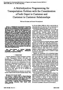
4.2.1 The Highest Effectiveness Approach (HEA) Sensitivity analysis are defined as recognizing the effect of individual input factors to uncertainty in the mathematical model calculations [25]. Input factors are dependent on numerous sources of uncertainty including errors of measurement, lack of information and partial understanding of the major causes and mechanisms. This uncertainty forces a limit on reliability of the model output. Moreover, models may be required to deal with the intrinsic variability of the system e.g. occurrence of stochastic events [26]. Uncertainty and Sensitivity Analysis provide valid tools for describing the uncertainty associated with a model. In order to do so, the Highest Effectiveness approach (HEA), is proposed:

Fig. 1 The Highest Effectiveness Approach (HEA) for Sensitivity Analysis

A Multi-Objective Programming Model for Disaster Preparedness Planning

51

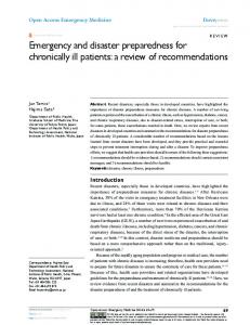
According to the proposed approach, the mathematical model is solved by a specific D with the ε-constraint method first, and some efficient solutions are generated. In other words, we assume that the occurrence time of the disaster (D) is equal to 1 and then the model is solved with this assumption and some efficient solutions are obtained.

Fig. 2 Solving the mathematical model for obtaining Pareto-front

The effectiveness index is computed separately for every solution of these obtained Paretooptimal solutions. To achieve this, an acceptable reliability and confidence rate is considered (e.g. 10%). Figure 3 and Figure 4 indicates the changing behavior of the parameter D against f1 (minimizing function) and f2 (maximizing function).

Fig. 3 Computing the L parameter and effectiveness of one solution with a specific D for the minimizing function (F1)

Fig. 4 Computing the L Parameter and effectiveness of one solution with a specific D for the maximizing function (F2)

52

M. Rabbani, et al. / IJAOR Vol. 5, No. 3, 41-57, Summer 2015 (Serial #17)

The parameter D is shifted and its behavior towards each function is investigated separately. The parameter L is calculated for each function and the effectiveness of the solution is computed as follows:   L / T F1   L / T F2  (23) Effectiveness  2 The solution which has the highest effectiveness is selected as the optimal solution for the specific D. the effectiveness is computed for all the possible D ( 1  D  T ) and the highest one among all is determined as the optimal solution.

5 Computational Results Due to the scarcity of the mathematical models in the preparedness context of disaster preparedness planning, no standard test problem has been generated. Therefore, to demonstrate the validity of the proposed model and the solution method, a hypothetical problem is generated in this paper. Assume a specific disaster like an earthquake is likely to happen during the next ten years in the region of the organization which we are planning (T  10 ). The organization has 5 important key functions (i.e. marketing, sales and customer service, accounting, telecommunications, public relationship communications) that are needed to be protected from any disruptions. These five functions are very important for the organization, because the potential costs of downtime for these functions (i.e. direct loss, lost future revenue, investment losses, damaged reputation and other expenses) are considerably high for the organization. Manager’s minimum satisfactory reliability level of the preparedness plan (  ) is 0.5 for these five functions. Organization’s budget allocation for the preparedness plan at the beginning of planning horizon ( B 0 ) is 1,000 monetary units and increases by 10% annually. As it was mentioned in section 3, each disaster will disrupt a particular set of key functions. In this case earth quake will disrupt sales and customer service, telecommunications and public relationship communications. Hence, the organizations’ functions matrix is assumed as follows: Ff   0 1 0 1 1 In order to be prepared for disaster, each of these functions needs a set of resources (i.e. backup facility, wireless communication systems, backup data storage devices) to recover in allowable disruption time. Required resources and the MADT to recover these functions are generated according to uniform distribution and presented in the Table 1. Table 1 Function’s related data

Function 1 2 3 4 5

r=1 U(0,2) U(0,2) U(0,2) U(0,2) U(0,2)

Resource r=2 U(1,3) U(1,3) 0 U(2,4) U(1,4)

r=3 U(20,70) U(50,150) U(100,200) 0 U(50,150)

MADT (h) U(100,200) U(100,150) U(200,300) U(100,120) U(100,170)

Four solutions were considered in this case and provided resources and execution times of using each resource are generated according to uniform distribution and presented in Table 2.

A Multi-Objective Programming Model for Disaster Preparedness Planning

53

Table 2 Solutions’ related data

Solution

Resource/Time(h) r=2 U(3,6)/U(40,60) U(6,10)/U(40,90) U(2,4)/U(20,40) U(2,5)/U(20,40)

1 2 3 4

r=1 U(1,2)/U(30,80) 0/0 U(1,3)/U(20,90) U(1,3)/U(20,90)

r=3 U(50,150)/U(5,15) U(200,500)/U(15,30) U(50,250)/U(5,25) 0/0

Cr 0

U(300,500)

U(40,80)

U(5,15)

MR r

U(2,6)

U(6,10)

U(700,1000)

According to historical data of the organization region, probability of the predicted time of disaster occurrence and probability of the predicted severity (Low, Medium, and High) of the disaster in each year is shown in Table 3. Table 3 Probability of the predicted time occurrence and the predicted severity of the disaster

Time period ( t )

0

Probability of occurrence ( Pt )

0

0.1 0.1 0.1 0.1 0.1 0.1 0.1 0.1 0.1 0.1

Cumulative probability

0

0.1 0.2 0.3 0.4 0.5 0.6 0.7 0.8 0.9

1

1)

0

0.9 0.8 0.8 0.1

0

M ( M

 1.2 )

0

0.1 0.2 0.1 0.8 0.8 0.7 0.6 0.2 0.1 0.1

H ( H

 1.5 )

0

Probability of Severity D

D

D

( P L , P M , P H )

L ( L

1

0

2

0

3

4

5

0

6

7

0

0

8

0

9

0

10

0.1 0.1 0.2 0.3 0.4 0.8 0.9 0.9

Based on an expert’s opinion the D,  and  parameters are calculated respectively as follows:  10  D    t .Pt  (24)  t 0     L .PDL   M .PDM   H .PDH (25) D   .  0.5 (26) T By using historical data of the organization’s region minimum acceptable rate of return (i) is 2.75% and predicted inflation rate is presented in table 4: Table 4 Predicted inflation rate

Time period ( t )

0

1

2

3

4

5

6

7

8

9

10

Inflation rate ( if t )

-

1.90%

1.15%

2.60%

3.70%

3%

2.10%

4%

4.30%

2.60%

2.70%

This test problem is solved with branch-and-bound (B&B) algorithm by using the LINGO 9.0 optimization software, which is executed on a Pentium 4, with Intel Core 2 Duo (2M Cache, 2.00 GHz, 800 MHz FSB) CPU processor using 2 GB of RAM. According to the augmented ε-constraint method, after finding ideal and nadir solutions for the second objective function, the range of second objective function is split into 4 point as follows. The table below shows the four different efficient solutions found for the test problem.

54

M. Rabbani, et al. / IJAOR Vol. 5, No. 3, 41-57, Summer 2015 (Serial #17)

Table 5 Computational results of the test problem

X fs

 2k  12  0.555

 22  0.703

 23  0.852

 24  1

s=1 0 1 0 1 1 0 0 0 1 1 0 1 0 1 1 0 1 0 1 1

f=1 f=2 f=3 f=4 f=5 f=1 f=2 f=3 f=4 f=5 f=1 f=2 f=3 f=4 f=5 f=1 f=2 f=3 f=4 f=5

s=2 0 0 0 0 0 0 0 0 0 0 0 0 0 0 0 0 0 0 0 0

Objective functions s=3 0 0 0 1 0 0 1 0 1 0 0 0 0 1 0 0 1 0 1 1

s=4 0 0 0 0 0 0 0 0 0 0 0 0 0 0 0 0 0 0 0 0

Cost

Reliability

3630

0.555

3634

0.703

3639

0.852

3643

1

The numbers in the Table 6 indicates the effectiveness of the four different efficient solutions found for the test problem. Table 6 The effectiveness for all the solutions

Solution

 12  0.555

 22  0.703

 23  0.852

 24  1

Effectiveness

0.5

0.5

0.3

0.3

Noted to the inconsiderable percentage of reliability, DM has preferred to select the cost criteria for performing the highest effectiveness effect and the threshold level for varying the cost is considered 0.4%. As the result of the HEA, the first solution is determined as the best solution with the cost of 3630 and reliability of 0.555. Figure 5 indicates the result of HEA for the selected solution.

Fig. 5 Highest Effectiveness diagram

A Multi-Objective Programming Model for Disaster Preparedness Planning

55

The cash flow for the preferred solution in the HEA is shown in Figure 6.

Fig. 6 Cash flow diagram

5.1. Sensitivity analysis Hereafter, the results of the proposed models must be verified and validated. To do so, 2 parameters are employed to perform a sensitivity analysis. Rate of return and initial cost of resources are selected by the decision maker and divided into 5 levels. The different surfaces of these parameters are shown in following tables: Table 7. 5 levels for initial cost of resources

Levels Initial cost of resources

r=1 r=2 r=3

1 350 30 3

2 400 40 4

3 450 50 5

4 500 60 6

5 550 70 7

Table 8. 5 levels for rate of return

Levels Rate of return

1 1%

2 2%

3 3%

4 4%

5 5%

After determining the different levels of the parameters, the proposed model is performed with these different levels. The result for the initial cost of resources parameters is illustrated in figure 7. The Figure indicates that the initial cost of resources and the first objective function are related directly. The initial cost of resources is investigated just with the first objective function because the relation of this parameter and second objective function is not significant. After analyzing the initial cost of resources parameter, rate of return is considered as the second parameter for performing the sensitivity analysis. Figure 8 and 9 indicate the result for the different levels of rate of return in the objective functions. The capability of model is confirmed with these results. When the rate of return increases, total cost (first objective function) decreases. However, reliability (second objective function) shows a stepped-

56

M. Rabbani, et al. / IJAOR Vol. 5, No. 3, 41-57, Summer 2015 (Serial #17)

behavior which is divided into transition and steady phases. According to the Figure 9 when rate of return increases, reliability remains steady (steady phase) until the constraints could not be satisfied.

Fig. 7 Sensitivity analysis of the first objective function (initial cost of resources)

Fig. 8 Sensitivity analysis of the first objective function (rate of return)

From then the reliability graph falls to another steady state (transition phase).

Fig. 9 Sensitivity analysis of the second objective function (rate of return)

6 Conclusions In this paper, a new multi-objective model for economic disaster preparedness planning under uncertainty is proposed. A two-step solution approach is developed to solve the proposed model. The numerical example shows applicability of the proposed model and solution approach. Sensitivity analysis on critical parameters validates the presented test problem and finally, obtained results find out a positive correlation between the vector of initial costs and first objective function. However, reliability of the most stable solutions does not indicate any significant correlation with this vector. As it was illustrated in figures 8 and 9 the objective functions show negative correlation with the rate of return parameter. Future research on this field can be concentrated on considering dependency of the key functions as an important assumption that affect the time of recovery plan.

A Multi-Objective Programming Model for Disaster Preparedness Planning

57

References 1. 2. 3. 4. 5. 6. 7. 8. 9. 10. 11. 12. 13. 14. 15. 16. 17. 18.

19. 20. 21. 22. 23.

24. 25. 26.

Pickren, A. (2012). The Concise Guide to Business Continuity Standards, MIR3 inc.. Hiles, Andrew. The definitive handbook of business continuity management. John Wiley & Sons, 2010. Staff, B. S. I. (2007). The Route Map to Business Continuity Management. Meeting the Requirements of BS 25999: B S I Standards. Hubbard, D. W. (2009). The failure of risk management: why it's broken and how to fix it: Wiley. Jenkins, L. (2000). Selecting scenarios for environmental disaster planning. European Journal of Operational Research, 121(2), 275-286. Tamura, H., Yamamoto, K., Tomiyama, S., Hatono, I. (2000). Modeling and analysis of decision making problem for mitigating natural disaster risks. European Journal of Operational Research, 122(2), 461-468. Bryson, K. M., Millar, H., Joseph, A., Mobolurin, A. (2002). Using formal MS/OR modeling to support disaster recovery planning. European Journal of Operational Research, 141(3), 679-688. Freeman, P. K. (2003). Infrastructure in developing and transition countries: Risk and protection. Risk Analysis, 23(3), 601-609. Okuyama, Y. (2003). Economics of natural disasters: A critical review.Research Paper, 12, 20-22. Okuyama, Y. (2008). Critical review of Methodologies on disaster impacts estimation. Background paper for EDRR report. Morris, S. S., Wodon, Q. (2003). The allocation of natural disaster relief funds: Hurricane mitch in honduras. World Development, 31(7), 1279-1289. Clower, T. L. (2005). Economic applications in disaster research, mitigation, and planning. Disciplines, Disasters and Emergency Management: The Convergence of Concepts Issues and Trends From the Research Literature. McEntire, D. A., Cope, J. (2004). Damage Assessment after the Paso Robles, San Simeon, California, Earthquake: Lessons for Emergency Management. Natural Hazards Center. Chang, S. E. (2003). Evaluating disaster mitigations: Methodology for urban infrastructure systems. Natural Hazards Review, 4(4), 186-196. Cochrane, H. (2004). Economic loss: Myth and measurement. Disaster Prevention and Management, 13(4), 290-296. Zimmerman, R. (2005). Electricity Case: Economic Cost Estimation Factors for the Economic Assessment of Terrorist Attacks. Center of Risk and Economic Analysis of Terrorism Events, University of Southern California, Los Angeles. McComb, R., Moh, Y. K., Schiller, A. R. (2011). Measuring long-run economic effects of natural hazard. Natural Hazards, 58(1), 559-566. Nakano, K., Kajitani, Y., Tatano, H. (2011). Consistent measurement of economic losses of a natural disaster considering the effect of change in price. IEEE International Conference on Systems, Man, and Cybernetics (SMC), 3489-3494. Park, J., Cho, J., Rose, A. (2011). Modeling a major source of economic resilience to disasters: Recapturing lost production. Natural Hazards, 58(1), 163-182. Mavrotas, G. (2009). Effective implementation of the ε-constraint method in Multi-Objective Mathematical Programming problems. Applied Mathematics and Computation, 213(2), 455-465. Dhaenens, C., Lemesre, J., & Talbi, E. G. (2010). K-PPM: A new exact method to solve multi-objective combinatorial optimization problems. European Journal of Operational Research, 200(1), 45-53. Esmaili, M., Amjady, N., Shayanfar, H. A. (2011). Multi-objective congestion management by modified augmented ε-constraint method. Applied Energy, 88(3), 755-766. Aghaei, J., Amjady, N., Shayanfar, H. A. (2011). Multi-objective electricity market clearing considering dynamic security by lexicographic optimization and augmented epsilon constraint method. Applied Soft Computing Journal, 11(4), 3846-3858. Haimes, Y. Y. (2011). Risk Modeling, Assessment, and Management: John Wiley & Sons. Lilburne, L., Tarantola, S. (2009). Sensitivity analysis of spatial models. International Journal of Geographical Information Science, 23(2), 151-168. Saltelli, A. (2008). Global Sensitivity Analysis: The Primer: John Wiley.