Sanja Petrovic and Yuri Bykov. School of Computer Science and Information Technology, ... especially for problems with a high number of criteria. Moreover, the.
A Multiobjective Optimisation Technique for Exam Timetabling Based on Trajectories Sanja Petrovic and Yuri Bykov School of Computer Science and Information Technology, University of Nottingham, Jubilee Campus, Nottingham NG8 1BB, UK {sxp, yxb}@cs.nott.ac.uk
Abstract. The most common approach to multiobjective examination timetabling is the weighted sum aggregation of all criteria into one cost function and application of some single-objective metaheuristic. However, the translation of user preferences into the weights of criteria is a sophisticated task, which requires experience on the part of the user, especially for problems with a high number of criteria. Moreover, the results produced by this technique are usually substantially scattered. Thus, the outcome of weighted sum algorithms is often far from user expectation. In this paper we suggest a more transparent method, which enables easier expression of user preferences. This method requires the user to specify a reference solution, which can be either produced manually or chosen among the set of solutions, generated by any automated method. Our aim is to improve the values of the reference objectives, i.e. to produce a solution which dominates the reference one. In order to achieve this, a trajectory is drawn from the origin to the reference point and a “Great Deluge” local search is conducted through the specified trajectory. During the search the weights of the criteria are dynamically changed. The proposed technique was experimentally tested on real-world exam timetabling problems on both bi-criteria and nine-criteria cases. All results obtained by the variable weights Great Deluge algorithm outperformed the ones published in the literature by all criteria.
1 1.1
Introduction Exam Timetabling Problems
University examination timetabling comprises arranging exams in a given number of timeslots. The primary objective of this process is avoiding students’ clashes (i.e. a student cannot take two exams simultaneously). This requirement is generally considered as a hard constraint and should be compulsory satisfied in a feasible timetable. However, a number of other restrictions and regulations,
180
Petrovic and Bykov
which depend on a particular institution, are also to be taken into account when solving exam timetabling problems. Some of them can be also considered as hard constraints, while other constraints are soft: i.e. usually they cannot be completely satisfied, and therefore their violations should be minimised. The soft constraints vary from university to university, as is shown in [2] where the authors analyse responses from over 50 British universities. The soft constraints usually imply the different importance of the timetable to the timetable officer (decision maker). They are generally incompatible and often conflict with each other. Timetabling problems can be considered to be multiobjective problems where objectives measure the violations of the soft constraints. We believe that multiobjective optimisation methods can bring new insight into timetabling problems by considering simultaneously different criteria during the construction of a timetable. 1.2
Multiobjective Optimisation of Examination Timetabling
The conventional challenge of multiobjective optimisation is assessment of the quality of solutions. Formally, one solution can be considered to be better than another only in the case when the values of all its criteria outperform those of the second ones: i.e. the first solution “dominates” the second one. All solutions which are not dominated by any other one, can be considered to be optimal. However, only one solution from this non-dominated set (often called the “Pareto front”) can become the final result. To obtain it, the decision maker must express his/her preferences. The group of multiobjective methods called “Search-then-Decide” (a posteriori) are designed to produce the set of non-dominated solutions from which the decision maker can select their preferable one. This approach is mostly applicable to small- and middle-sized combinatorial optimisation problems. To our knowledge, there are no publications about the use of these methods for examination timetabling. However, several authors (for example [9, 17]) have applied a posteriori algorithms to class–teacher timetabling, a problem which is similar to examination timetabling. Traditionally, exam timetabling problems are solved by the “Decide-thenSearch” (a priori) approach. In these methods the decision maker specifies his/her preferences regarding the solution before launching the algorithm. The most popular method involves aggregation of the problem’s objectives into a cost function in order to apply some single-objective metaheuristic (see survey [8]). Usually, the cost is calculated as a weighted sum of objectives. This method has been applied with simulated annealing [15, 16], tabu search [1], genetic algorithms [10], a memetic algorithm [4], etc. In another method, lexicographic ordering, criteria are divided into groups and the search is conducted in several phases by each group. This method has been applied to the examination timetabling by several authors [12, 14]. In [5] the authors investigated a Compromise Programming technique with different distance measures as the means of aggregation of an objective’s values while applying the search algorithm, designed as a hybrid of heavy mutation and hill-climbing.
Multiobjective Optimisation
181
Set the initial solution s0 Calculate the initial cost function f (s0 ) Initial level B0 = f (s0 ) Specify the input parameter ∆B = ? While not some stopping condition do Define neighbourhood N (s) Randomly select the candidate solution s∗ ∈ N (s) If (f (s∗ ) ≤ f (s)) or (f (s∗ ) ≤ B) Then accept s∗ (s = s∗ ) Lower the level B = B − ∆B Fig. 1. Single-objective Great Deluge algorithm
1.3
Great Deluge
Great Deluge is a local search metaheuristic, introduced by Dueck [11]. In [6] the authors showed its quite promising performance on exam timetabling problems. In this algorithm a new candidate solution (selected from a neighbourhood) is accepted if its objective function is either not worse than a current one or does not exceed the current upper limit B (level ). The value of the level is reduced gradually throughout the search by some specified decay rate ∆B, which denotes the search speed. Decrease of the level forces the current solution’s cost function to correspondingly decrease until convergence. The initial value of B is equal to the cost function of the initial solution, and therefore no additional parameters are required. The pseudocode of the basic variant of the Great Deluge algorithm is given in Figure 1. Having the search speed as an input parameter leads to the unique property of this algorithm. It provides two options: either the decision maker can estimate beforehand the processing time from the start to the convergence, or alternatively, the value of ∆B can be calculated in order to fit the search into a certain predefined time interval. Experiments with this technique have shown that a longer search usually yields a better final result, and this principle achieves its full strength when applied to large-scale timetabling problems. With the Great Deluge algorithm the decision maker can obtain higherquality results at the price of prolongation of the search period (this is viable because processing time is usually not an issue in exam timetabling problems). The algorithm allows him/her to choose a preferable balance between the quality of the solution and the searching time, to fit a solving procedure into his/her personal schedule and to optimise the utilisation of computational resources. In [6] and [7] we presented a comprehensive comparison of the Great Deluge algorithm with a variety of useful metaheuristics on different benchmark problems. In almost all the experiments our approach outperformed the other metaheuristics. In this paper we present a modified Great Deluge algorithm for multiobjective timetabling problems. The paper is organised in the following way. Section 2 gives the description of the reference points and trajectories in the criteria space. In
182
Petrovic and Bykov
Section 3 we introduce the variable weights multiobjective extension of the Great Deluge algorithm. Results of the experiments are given in Section 4. Finally, in Section 5 we summarise our contribution and suggest directions for future work.
2
Reference Solution in Criteria Space
The general drawback of the weighted sum approach is the necessity of defining particular values of weights. This requires experience on the part of the decision maker. The translation of his/her preferences into the form of weights is a sophisticated task, especially for problems with a high number of criteria. Furthermore, the results produced by the weighted sum are usually substantially scattered. Thus, the weighted sum technique often produces an outcome that is far from the decision maker’s expectations. Often, the proper setting of weights can be done only by launching the search procedure several times. As an alternative to the traditional weighted sum approach we expand the idea of reference timetable expressed by Paechter et al. [13]. As the reference they considered a timetable produced either manually or automatically using another dataset. The authors suggested an algorithm which obtains a solution genotypically similar to the reference one. They also pointed out that the reference solution may already be located in a local optimum, and therefore it is worth starting the search for the new solution from scratch. For the purpose of multiobjective optimisation the reference solution can be considered in a phenotypic sense: i.e. the decision maker should specify the criteria values of some attainable solution which to a certain degree meet his/her preferences. This solution can be produced manually or selected from the set of solutions generated by some automated method. We assume that the decision maker is not satisfied completely with this solution, but this choice gives information that is helpful for a further search for a better solution. Having a more or less preferable reference solution, we can consider that all further solutions which dominate the reference one (where all reference criteria are outperformed by the new ones) will be even more preferable. In order to find these solutions, we suggest the following method. We represent the reference solution as a point in the criteria space and draw a line through this point and the origin. When the search procedure is launched, an initial solution and all the following current solutions are also represented as points in the criteria space. The algorithm should provide the gradual improvement of the current solution while keeping the corresponding points close to the defined line. The aim is to approach as close to the origin as possible, driving the search through the defined trajectory. In our approach the reference solution is used only for drawing the trajectory, but does not affect the further search process. We use it only as a benchmark for assessing the final solution. As the reference solution in most cases already lies in a local optimum, it cannot be used for the initialisation purpose. Generally, local search techniques show the best performance when they start from a random solution. Therefore. we suggest keeping this practice for the presented approach.
Multiobjective Optimisation
183
c2 I
R c1
0 Fig. 2. Following the defined trajectory
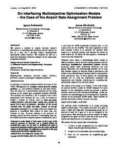
For the bi-criteria case the method is illustrated in Figure 2, where the trajectory is depicted as a dash-dotted line. The search starts from a randomly generated initial solution (point I) and at first approaches the trajectory (generally, the initial solution does not lie on the trajectory). The search then follows the trajectory until it reaches the vicinity of the reference solution (point R) and continues along it until convergence. In the final stage any solution dominates the reference one. The point of convergence is not known in advance, but it will be obviously superior to the reference point.
3
Great Deluge with Variable Weights
In this section we present a technique suitable for driving the search through a predefined trajectory. It operates with a weighted sum cost function, but the weights are varied dynamically during the search. We have developed a special procedure for weight variation to regulate the direction of the search. The explanation of our method is illustrated with a bi-criteria case (the goal is to minimise criteria c1 and c2 ). We consider a weighted sum aggregation function with weights w1 and w2 within the Great Deluge algorithm. The condition of acceptance of a candidate solution S = (s1 , s2 ) at any iteration can be expressed by the following inequality: s1 w1 + s2 w2 ≤ B .
(1)
This formula states that the algorithm accepts any solution in the space bounded by axes c1 and c2 (as the criteria values are always positive) and the line c1 w1 + c2 w2 = B .
(2)
184
Petrovic and Bykov
c2 G2 G2
*
S* 0
S c1 G1
*
G1
Fig. 3. Borderline in the weighted sum Great Deluge algorithm
In Figure 3 this borderline is marked as G1 G2 . The points where it intersects the axes can be calculated as G1 = B/w1 ; G2 = B/w2 . The space of acceptance is denoted by the shaded triangle. The lowering of the level value B at each step corresponds to a shift of the borderline towards the origin. The new borderline G1 ∗ G2 ∗ is expressed by c1 w1 + c2 w2 = B − ∆B . G∗1
(3) G∗2
= (B − ∆B)/w1 and = The new intersection points are calculated as (B − ∆B)/w2 . The shifting of the borderline results in obtaining the new current solution (S ∗ ) which is closer to the origin. Let us define ∆w = ∆w/(B − ∆B), and equation (3) can be transformed into the following form: c1 w1 (1 + ∆w) + c2 w2 (1 + ∆w) = ∆B .
(4)
Due to this formula the decrease of the level at any given iteration can be replaced with the appropriate increase of both weights as it causes the same effect (shifting of the borderline). Hence, finally, each separate increase of a single weight induces a rotation of the borderline such that the new solution improves the corresponding criterion more than the other one. Thus, equation (5) corresponds to the line G∗1 G2 in Figure 4 and equation (6) corresponds to the line G1 G∗2 in Figure 5: c1 w1 (1 + ∆w) + c2 w2 = ∆B , c1 w1 + c2 w2 (1 + ∆w) = ∆B .
(5) (6)
For example, the increase of w1 in Figure 4 forces solution S to move mostly along the c1 axis. The increase of w2 causes the opposite effect (Figure 5). Thus, instead of reducing a level at each step, the proposed algorithm increases a single weight. Although the value of level B is invariable, we can con-
Multiobjective Optimisation
c2 G
S
*
S c1
0
G1
*
G1
Fig. 4. The increase of w1
c2 G2 G2
*
S *
S
c1 0
G1 Fig. 5. The increase of w2
185
186
Petrovic and Bykov
c2 t1/r1< t2/r2 t1/r1= t2/r2 S’(s1’,s2’) R (r1,r2)
0
t1/r1> t2/r2
S”(s1”,s2”)
c1
Fig. 6. The selection of increased weight
sider this technique as a multiobjective extension of the Great Deluge algorithm because it incorporates the same principles. In order to force the current solutions to follow the given trajectory, the algorithm employs the appropriate rule for selecting the weight to be increased. We suggest the following method (its bi-criteria case is illustrated in Figure 6). As the trajectory (dash-dotted line) is drawn through the reference point R = (r1 , r2 ) and the origin, then any point (t1 , t2 ), where t1 /r1 = t2 /r2 , belongs to the trajectory. Thus, the trajectory divides the criteria space into two halves: one where t1 /r1 < t2 /r2 and the other where t1 /r1 > t2 /r2 . Obviously, if point S � (the current solution) is placed in the first half (above the trajectory), the directing of the search towards the trajectory can be done while decreasing s�2 (increasing w2 ). In the other half (below the trajectory), for point S �� we have to increase w1 . The proposed rule can be expanded into n-criteria space as well. Here, we evaluate the vector (s1 /r1 , s2 /r2 , . . . , sn /rn ), choose its maximum element and increase the corresponding weight. The pseudocode of the algorithm is given in Figure 7. In this algorithm the value of the input parameter ∆w affects the computing time in the sense that with higher ∆w the search runs faster. However, in contrast to the basic single-objective variant, the search speed is not steady, and therefore we cannot guarantee convergence in the given number of iterations. We expect that this could be arranged with a more advanced mechanism of weight variation. Additionally to ∆w, this algorithm requires the specification of initial weights (w10 , w20 , . . . , wi0 ). Their relative proportion defines the angle of an initial borderline, which passes through the initial solution. We have experimentally tested different methods of weight initialisation and found that they affect the duration of the first phase of the search: proper definition of initial weights allows the current solution to reach the trajectory more expeditiously. The best values of initial weights are probably problem dependent. However, in our experiments a fairly good performance was achieved when setting w10 equal to s01 /ri . If the value of some reference criterion ri is equal to 0 (the constraint in the reference
Multiobjective Optimisation
187
Set the reference solution R = (r1 , r2 , . . . , rn ) Set the initial solution S 0 = (s01 , s02 , . . . , s0n ) Specify the initial weights (w10 , w20 , . . . , wn0 ) = ? Calculate initial cost function f (S) = s01 w10 + s02 w20 + · · · + s0n wn0 level B = f (S) Specify the input parameter ∆w = ? While not stopping condition do Define a neighbourhood N (S) Randomly select the candidate solution S ∗ ∈ N (S) If (f (S ∗ ) ≤ f (S)) or (f (S ∗ ) ≤ B) Then accept candidate S = S ∗ Find i corresponding to: maxi=1...n (si /ri ) Increase the weight wi = wi (1 + ∆w)
Fig. 7. Multiobjective Great Deluge algorithm with variable weights
solution is satisfied), we put, instead of ri , some small value which is less than half of the measurement unit of the criterion. For example, when the criterion has integer value, it is enough to set ri = 0.4.
4
Experiments
The proposed algorithm was experimentally tested on real-world large-scale examination timetabling data. The algorithm was implemented on C++ and launched on PC with AMD Athlon 750 MHz processor under OS Windows98. 4.1
Bi-criteria Case
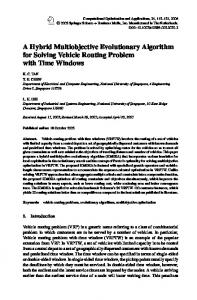
The first series of experiments was done on a bi-criteria case. We used the following university examination timetabling datasets: the University of Nottingham dataset (Nott-94), placed at ftp://ftp.cs.nott.ac.uk/ttp/Data/Nott94-1, and two datasets (Car-f-92 and Kfu-s-93) from the University of Toronto collection, available at ftp://ftp.mie.utoronto.ca/pub/carter/testprob. The problem formulation was the same as in [4]: the first objective represents the number of conflicts where students have to sit two exams in adjacent periods, and the second objective represents the number of conflicts where students have exams in overnight adjacent periods. In our first experiment we investigated the ability of the presented technique to follow a defined trajectory. For the Nott-94 problem we specified both reference criteria values to be equal to 300. The trajectory is a line under the 45◦ angled line (dash-dotted line in Figure 8), and ∆w was set to be 10−6 (processing time was around 3 min). In order to follow the progress of the search process, we plotted after each 50 000 steps the current solution as a dot and after each
188
Petrovic and Bykov Table 1. Reference and our solutions for the bi-criteria case Car-f-92 (36 periods) MSMA TBA 1st point
C1 C2 C1 C2 C1 C2
302 804 313 766 363 576
282 799 286 706 327 541
Kfu-s-93 (21 periods) MSMA TBA 222 838 228 704 307 589
204 743 218 608 258 562
Nott-94 (23 periods) MSMA TBA 65 324 76 282 100 255
53 271 57 187 59 149
500 000 steps we drew the current borderline as a dotted line. The complete diagram is presented in Figure 8. The search is first directed towards the trajectory and then follows it producing solutions, which are very close to it. Scatter is relatively high at the beginning of the search and then becomes very low. Looking at the dynamics of the borderline we can notice that at the beginning of the search only w1 has been increasing until the current solution reaches the trajectory. After that, the two weights increase differently, using the rules described in Section 3. The second series of experiments were done using published results as reference points. We used the results produced by the Multi-Stage Memetic algorithm presented in [4], while using the same weighted sum cost function. We selected from the best presented results three non-dominated points for every dataset (marked as MSMA in Table 1). The corresponding trajectory was drawn for every reference point. Each launch of our trajectory-based algorithm was started from a random solution and lasted around 30–40 min. Approximately 95% of this time was spent on approaching the reference point and 5% on its improvement. Our final results are shown in Table 1 and marked as TBA. All our final results dominate the corresponding reference points. This confirms the ability of our algorithm to drive the search through different trajectories, and to produce high-quality solutions, which are better than the reference ones. 4.2
Nine-Criteria Case
We conducted the next series of experiments in order to investigate the effectiveness of the proposed technique when the number of criteria is greater than two. The Nott-94 dataset was considered with nine objectives in the same way as in [5]. Descriptions of the criteria are given in Table 2. Again we use the solutions presented in [5] as reference points. They were obtained by the multiobjective hybrid of heavy mutation and hill-climbing based on the idea of the Compromise Programming approach. These solutions were produced with different aggregation functions while scheduling exams into 23,
Multiobjective Optimisation
Fig. 8. The progress diagram for the Nott-94 problem
Table 2. Descriptions of criteria Criterion
Description
C1 C2
Number of times that room capacities are exceeded Number of conflicts, where students have exams in adjacent periods on the same day Number of conflicts, where students have two or more exams in the same day Number of conflicts, where students have exams in adjacent days Number of conflicts, where students have exams in overnight adjacent periods Number of times that students have exams that are not scheduled in period of proper duration Number of times that students have exams that are not scheduled in the required time period Number of times that students have exams that are not scheduled before/after another specified exams Number of times that students have exams that are not scheduled immediately before/after another specified exams
C3 C4 C5 C6 C7 C8 C9
189
190
Petrovic and Bykov Table 3. Reference and our solutions for nine-criteria case
Point 1st
2nd
3rd
C1 C2 C3 C4 C5 C6 C7 C8 C9 C1 C2 C3 C4 C5 C6 C7 C8 C9 C1 C2 C3 C4 C5 C6 C7 C8 C9
23 periods CPA TBA
26 periods CPA TBA
29 periods CPA TBA
32 periods CPA TBA
1038 1111 3518 4804 405 4 – – – – 879 3623 6381 264 – – – – 2848 2608 4886 4658 807 170 40 – –
137 655 2814 2759 265 – – – – – 604 2544 4571 164 – – – – 2044 1872 3507 3343 475 119 24 – –
139 513 2239 2172 231 – – – – – 393 1957 3438 151 – – – – 1559 1435 2688 2563 441 89 24 – –
25 314 1546 1646 174 – – – – – 316 1332 2482 53 – – – – 1243 1138 2132 2033 334 74 18 – –
795 651 3360 4185 54 – – – – – 778 3524 6221 152 – – – – 1734 1367 3760 2289 332 0 – – –
0 476 2795 2494 45 – – – – – 353 2174 3661 38 – – – – 889 802 2127 1922 190 – – – –
0 360 2059 1687 43 – – – – – 292 1482 2518 48 – – – – 670 703 1481 1201 128 – – – –
0 184 1353 1390 104 – – – – – 190 1104 2028 2 – – – – 1 488 1210 1073 155 – – – –
26, 29 and 32 periods. The processing time of each launch was in the range of 5–10 min and any attempt to increase the processing time did not lead to better results. The presented trajectory-based technique was launched for each of these reference points. Our launches lasted approximately 20–25 min and we consider this processing time to be quite acceptable for examination timetabling. The results are compiled in Table 3. As in the previous experiments, the algorithm produces solutions which dominate the reference ones by all criteria. Thus, the proposed technique provides better satisfaction of user preferences as well as higher overall result quality than conventional weighted sum methods.
Multiobjective Optimisation
5
191
Conclusions and Future Work
In this paper we have presented a new multiobjective approach, whose main characteristics are as follows: – instead of reducing the aggregation function, our algorithm aims to improve each criterion separately by changing weights dynamically during the search process; – the specification of a reference solution may be more transparent to the decision maker than expressing the weights; – the final solution produced by the algorithm conforms to the reference one, which satisfies the decision maker’s preferences. Therefore, it is expected to be more acceptable to the decision maker; – the solutions dominate the results of other techniques. Therefore, the presented approach can be considered to be a more powerful one. This paper opens a wide area for further research. The proposed algorithm should be evaluated in other domains, with different numbers of objectives. Different procedures for weight variation could be developed, to direct the search differently. In particular, the question of weight initialisation needs further investigation. In addition, other approaches to trajectory definition should be explored.
References 1. Boufflet, J.P., Negre, S.: Three Methods Used to Solve an Examination Timetabling Problem. In: Burke, E, Ross, P. (Eds.): Practice and Theory of Automated Timetabling I (PATAT’95, Edinburgh, Aug/Sept, selected papers). Lecture Notes in Computer Science, Vol. 1153. Springer-Verlag, Berlin Heidelberg New York (1996) 327–344 2. Burke, E.K., Elliman, D.G., Ford, P.H., Weare, R.F.: Examination Timetabling in British Universities: a Survey. In: Burke, E, Ross, P. (Eds.): Practice and Theory of Automated Timetabling I (PATAT’95, Edinburgh, Aug/Sept, selected papers). Lecture Notes in Computer Science, Vol. 1153. Springer-Verlag, Berlin Heidelberg New York (1996) 76–90 3. Burke, E.K., Jackson, K., Kingston, J.H., Weare, R.: Automated University Timetabling: The State of the Art. Comput. J. 40 (1997) 565–571 4. Burke, E.K., Newall, J.P.: A Multi-stage Evolutionary Algorithm for the Timetabling Problem. IEEE Trans. Evolut. Comput. 3 (1999) 63–74 5. Burke, E.K., Bykov, Y., Petrovic, S.: A Multicriteria Approach to Examination Timetabling. In: Burke, E, Erben W. (Eds.): Practice and Theory of Automated Timetabling III (PATAT 2000, Konstanz, Germany, August, selected papers). Lecture Notes in Computer Science, Vol. 2079. Springer-Verlag, Berlin Heidelberg New York (2001) 118–131 6. Burke, E.K., Bykov, Y., Newall, J.P., Petrovic, S.: A Time-Predefined Local Search Approach to Exam Timetabling Problems. Computer Science Technical Report NOTTCS-TR-2001-6, University of Nottingham (2001)
192
Petrovic and Bykov
7. Burke, E.K., Bykov, Y., Newall, J.P., Petrovic, S.: A New Local Search Approach with Execution Time as an Input Parameter. Computer Science Technical Report NOTTCS-TR-2002-3, University of Nottingham (2002) (to appear in Proc. 6th Balkan Conf. Oper. Res.) 8. Carter, M.W., Laporte, G.: Recent Developments in Practical Examination Timetabling. In: Burke, E, Ross, P. (Eds.): Practice and Theory of Automated Timetabling I (PATAT’95, Edinburgh, Aug/Sept, selected papers). Lecture Notes in Computer Science, Vol. 1153. Springer-Verlag, Berlin Heidelberg New York (1996) 3–21 9. Carrasco, M.P., Pato, M.V.: A Multiobjective Genetic Algorithm for the Class/Teacher Timetabling Problem. In: Burke, E, Erben W. (Eds.): Practice and Theory of Automated Timetabling III (PATAT 2000, Konstanz, Germany, August, selected papers). Lecture Notes in Computer Science, Vol. 2079. Springer-Verlag, Berlin Heidelberg New York (2001) 3–17 10. Corne, D., Ross, P., Fang, H.L.: Fast Practical Evolutionary Timetabling. In: Fogarty, T.C.: Proc. AISB Workshop Evolut. Comput. (1994) 250–263 11. Dueck, G.: New Optimization Heuristics. The Great Deluge Algorithm and the Record-to-Record Travel. J. Comput. Phys. 104 (1993) 86–92 12. Lotfi, V., Cerveny , R.: A Final-Exam Scheduling Package. J. Oper. Res. Soc. 42 (1991) , 205–216 13. Paechter, B., Rankin, R.C., Cumming, A., Fogarty, T.C.: Timetabling the Classes of an Entire University with an Evolutionary Algorithm. In: Parallel Problem Solving from Nature (PPSNV) Springer-Verlag, Berlin Heidelberg New York (1998) 14. Thompson, J.M., Dowsland, K.A.: Multi-Objective University Examination Scheduling. EBMS/1993/12, European Business Management School, University of Wales, Swansea (1993) 15. Thompson, J.M., Dowsland, K.A.: Variants of Simulated Annealing for the Examination Timetabling Problem. Ann. Oper. Res. 63 (1996) 105–128 16. Thompson, J.M., Dowsland, K.A.: A Robust Simulated Annealing Based Examination Timetabling System. Comput. Oper. Res. 25 (1998) 637–648 17. Tanaka, M., Adachi, S.: Request-Based Timetabling by Genetic Algorithm with Tabu Search. 3rd Int. Workshop Frontiers Evolut. Algorithms (2000) 999–1002