Department of Applied Mathematics
P.O. Box 217 7500 AE Enschede The Netherlands
Faculty of EEMCS
t
University of Twente The Netherlands
Phone: +31-53-4893400 Fax: +31-53-4893114 Email:
[email protected] www.math.utwente.nl/publications
Memorandum No. 1728 A multiple-choice knapsack based algorithm for CDMA downlink rate differentiation under uplink coverage restrictions A.I. Endrayanto, A.F. Bumb and R.J. Boucherie
July, 2004
ISSN 0169-2690
A multiple-choice knapsack based algorithm for CDMA downlink rate differentiation under uplink coverage restrictions A. Irwan Endrayanto, Adriana F. Bumb and Richard J.Boucherie Stochastic Operations Research, Department of Applied Mathematics, University of Twente, P.O.Box 217, 7500 AE Enschede, the Netherlands. {a.i.endrayanto, a.f.bumb, r.j.boucherie}@ewi.utwente.nl Abstract This paper presents an analytical model for downlink rate allocation in Code Division Multiple Access (CDMA) mobile networks. By discretizing the coverage area into small segments, the transmit power requirements are characterized via a matrix representation that separates user and system characteristics. We obtain a closed-form analytical expression for the so-called PerronFrobenius eigenvalue of that matrix, which provides a quick assessment of the feasibility of the power assignment for a given downlink rate allocation. Based on the Perron-Frobenius eigenvalue, we reduce the downlink rate allocation problem to a set of multiple-choice knapsack problems. The solution of these problems provides an approximation of the optimal downlink rate allocation and cell borders for which the system throughput, expressed in terms of downlink rates, is maximized. Keyword: CDMA, transmit power feasibility, Perron-Frobenius eigenvalue, border optimization, downlink rate allocation. AMS Subject Classification: Primary: 90B18, 90B22; Secondary: 60K25
1
Introduction
In Code Division Multiple Access (CDMA) systems, transmissions of different terminals are separated using (pseudo) orthogonal codes. The impact of multiple simultaneous calls is an increase in the interference level, that limits the capacity of the system. The assignment of transmission powers to calls is an important problem for network operation, since the interference caused by a call is directly related to the power. In the CDMA downlink, the transmission power is related to the downlink rate. Hence, for an efficient system utilization, it is necessary to adopt a rate allocation scheme in the transmission powers assignment. The rate assignment problem has been extensively studied in the literature [4, 8, 14, 18, 20]. In [8], a joint power and multiclass rate allocation algorithm for the uplink is considered. The problem is formulated as a non-linear optimization problem that is solved in two steps. In the first step, one decides for each user a SIR level that guarantees a maximum system utility. In the second, the SIR levels obtained are used to determine an optimal rate allocation. In [14] several rate assignments are analyzed in the context of the trade-off between fairness and over-all throughput. The algorithms presented in [8] and [14] find a solution to the rate optimization problem via the Lagrangian dual. Another approach for joint optimal rates and powers allocation, based on Perron-Frobenius theory, is presented in [4] and [18]. [4] presents a distributed algorithm for assigning base station transmitter (BTSs) powers such that the common rate of the users is maximized, while in [18] multiple rates are considered. [10] develops a model for characterizing downlink and uplink power assignment feasibility based on the Perron-Frobenius theory. It is shown that the transmission power assignment problem can be translated into the border location optimization problem, where these optimization problems for the downlink rate and optimal cell border take into account both uplink and downlink feasibility.
1
Based on the result in [10], in this paper we extend the model towards a downlink multi-rate allocation scheme. We study transmission power feasibility and data rate allocation problem for CDMA networks that supports variable transmission rate. The objective is to derive an analytical model and to develop an algorithm for downlink rate allocation with variable transmission rates. Moreover the model is used to determine an optimal cell border by taking into account both uplink and downlink feasibility. Our approach for the downlink rate allocation algorithm is based on the Perron-Frobenius eigenvalue of a power assignment related matrix that allows us to determine first the cell border location and then a near to optimal rate allocation. We call a rate allocation optimal if it maximizes the system utility. We show that the rate allocation problem can be reduced to a set of multiple choice knapsack problems for which efficient algorithms are known. Based on Fully Polynomial Time Approximation Scheme (FPTAS) for the multiple choice knapsack problems, we are able to design a FPTAS for the rate allocation problem. Hence, for an ² > 0, our algorithm returns an allocation of value at least (1 − ²)∗optimum in polynomial time in the size of the input data and (1/²). The remainder of this paper is organized as follows. We present the downlink interference and feasibility model in Section 2. The downlink rate allocation algorithm and a combined down- and uplink capacity allocation model are presented in Section 3. In Section 4 we present the numerical results and we conclude our work in Section 5.
2
Model
This paper focuses on the modeling of downlink rate allocation in a CDMA system consisting of BTSs located along a highway. Specifically, we focus on a two cell model, where only the area in between two base stations is taken into account. The description can readily be generalized to larger networks.
2.1
Cell Model
Consider a cell model as presented in [10]. We focus on modeling BTSs located along a highway to include both non-homogeneity of the call distribution, and mobility of calls. Users are located in cars passing through the cells. Due to e.g. traffic jams (”hot spots”) the load of the cells will not be distributed evenly along the road. To characterize the distribution of a single type of calls in the cells, we propose a discretized-cell model. Each cell is divided into small segments. Then, the nonhomogeneous load can be characterized by the mean number of calls and fresh call arrival rates in the segments. Taking into account interference between segments in neighboring cells and between segments within the cells, we express the generated downlink interference per segment towards the other segments. We consider a linear network model consisting of two BTSs, X and Y, say. Let the area between these BTSs be divided into segments of length δ. For the description below, we fix the radii of the cells. Let cell X contains I segments, labelled as i = 1, ..., I, and let cell Y contains J segments, labelled as j = 1, ..., J. Then L1 = Iδ is the radius of cell X, see Figure 1. Let D = δ(I + J), the distance between the BTSs. CELL BORDER
BTS X 1 2
i-1
i
I
BTS Y
j-1
J
segment i
i-1
i*
j
2 1
segment j
i
j-1
CELL RADIUS L1
j*
j
CELL RADIUS L2
Fig.1. Discretized Cell Model
We assume that the segments are small, so that we may approximate the location of terminals in a segment to be in the middle of that segment, i.e. for segment i of cell X, users are located at distance i∗ = δ [(i − 1) + i] /2 from X. Furthermore, we consider a deterministic Okumura-Hata path loss propagation model between a transmitter and a receiver, which performs reasonably in flat service areas (see [1, 12]): Pi = P0 (di )−γ ,
(1)
where Pi is the received power, P0 is the transmitted power, di is the distance between transmitter and receiver and γ the path loss exponent.
2.2
Downlink Interference Model
For the discretized cell model, we consider the downlink interference model proposed in [10]. Assume that the number of terminals in each segment in both BTSs is known. Let UX = (n1 , n2 , · · · , nI ) be a vector representing the number of terminals connected to BTS X, where ni is the number of terminals in segment i = 1, 2, · · · , I; and let UY = (m1 , m2 , · · · , mJ ) be a vector representing the number of terminals connected to BTS Y, where mj is the number of terminals in segment j = 1, 2, · · · , J. Furthermore, let X = (X1 , X2 , · · · , XI ) and Y = (Y1 , Y2 , · · · , YJ ) be the transmit power vectors of BTS ³ ´ X and BTS Y to terminals in the segments. Then, the energy per bit to interference ratio, Eb I0 , for a terminal i ∈ {1, 2, · · · , I} is defined as (see e.g. [13]) µ
Eb I0
¶ = i
W Xi (i∗ )−γ , ri Iintracell + Iintercell + N0
(2)
where W is the system chip rate,µ ri is the data¶rate, Iintracell is the interferences from users within I P the cell, i.e. Iintracell = α (i∗ )−γ nl Xl − Xi with α is non-orthogonality factor, Iintercell is the l=1
interferences from users in neighboring cell, i.e. Iintercell = (D − i∗ )−γ
J P
mj Yj , and N0 is the thermal
j=1
noise. A similar expression to (2) holds for j ∈ {1, 2, · · · , J} . For a terminal i ∈ {1, 2, · · · , I} , downlink transmission at sufficient quality requires the energy per bit to interference ratio to exceed a certain threshold ²∗iD , i.e., a terminal in segment i requires BTS X to transmit enough power such that µ ¶ Eb > ²∗iD , for i ∈ {1, 2, · · · , I} , (3) I0 i and similarly for a terminal segment j requires BTS Y to transmit enough power such that µ ¶ Eb > ²∗jD , for j ∈ {1, 2, · · · , J} . I0 j
(4)
We assume that the ( EI0b )−target is the same, i.e., ²∗iD = ²∗jD = ²∗D for all i = 1, 2, · · · , I and j = 1, 2, · · · , J. The model can be easily extended to different ( EI0b )−target. Under the quality of service (QoS) constraints, we are interested in finding a downlink rate assignment such that there exist non negative transmit power vectors X and Y satisfying (3). Without loss of generality, in this paper we assume that all users in the same segment have the same rate ri chosen from a finite set of possible transmission rates Ri ⊆ {r1 , r2 , · · · , rK }. Note that, if in a segment the maximum rate rK is not requested, then Ri ⊂ {r1 , r2 , · · · , rK } . This assumption leads to a better use of the resources. Let RX = (r1 , r2 , · · · , rI ) , respectively RY = (r1 , r2 , · · · , rJ ) , be the rates assigned to terminals in cell X, respectively cell Y.
Under the assumption of perfect power control, (3) becomes: I J X X Xi = αVi ni Xi + Vi pi mj Yj + Vi N0 di , i=1
for i = 1, 2, · · · , I,
(5)
j=1
where ²∗D ri ; Vi = W + α²∗D ri
µ pi =
D − i∗ i∗
¶−γ
µ ¶−γ 1 and di = ∗ , i
for i = 1, 2, · · · , I.
(6)
(5) express the required BTS X transmit powers to all segment i, i = 1, 2, · · · , I. Similarly, we can write the required BTS Y transmit powers to all segment j, j = 1, 2, · · · , J, in the cell Y. Thus system (3) and (4) can be rewritten in matrix form as follows (I − T)ZD = c. where ZD =
³ ´ (Xi )i=1,2,··· ,I , (Yj )j=1,2,··· ,J is the transmit powers vector;
µ
(7) 
VX DX VY DY = (di )i=1,2,··· ,I and
c =N0
with diagonal matrices VX = diag(Vi ) and VY = diag(V¯j ), and vectors DX DX = (dj )j=1,2,··· ,J given by (6); and the square matrix µ ¶µ ¶µ ¶ VX 0 α1X PX N 0 T= . (8) 0 VY PY α1Y 0 M ¡ D−i∗ ¢−γ X where PX = (pX is a matrix of size I × J that represents the inter-cell path loss ij ), pij = i∗ ´ ³ ∗ −γ ; the square from segment j in cell Y and segment i in cell X, and PY =(pYji ), where pYji = D−j ∗ j matrices N = UX I and M = UY I give the distribution of users. System (7) is the downlink power control equation. Since matrix T is a non-negative matrix, we can use the Perron-Frobenius theory to characterize the feasibility of (7). Thus, given the number of terminals in each cell UX and UY and the current rate allocation RX and RY , we can verify whether a feasible transmit power solution exists. This will be described in the next section.
2.3
Downlink Feasibility
According to the Perron-Frobenius theorem (see [19]), the feasibility of (7) is determined by the Perron- Frobenius (PF) eigenvalue λ (T) of the matrix T, i.e., ZD ≥0 exist
and ZD = (I − T)−1 c ⇐⇒ λ(T) < 1.
(9)
Hence, downlink transmit power feasibility is completely characterized by the matrix T given in (8). Characterization (9) provides a clear motivation for discretization. By discretizing the cell into segments, we obtain an analytical model for characterizing the transmit power feasibility for a certain rate allocation and a certain users distribution. We obtain a downlink interference model that is very similar to uplink models such as studied in [3, 9, 11] where feasibility of the uplink power control algorithm is characterized via the Perron-Frobenius (PF) eigenvalue of a matrix containing the number of calls in the cell (not in segments). The explicit expression of the PF eigenvalue has been derived for the case ri = rj = RD for all i and j (see [10]). The result can be extended to the case of different rates. For this purpose, we do a dimension reduction of the power control matrix, as was done for the uplink (see [11, 16, 22]). The following lemma provides a proof for the dimension reduction of matrix (8). Lemma 1 System (7) is feasible if and only if the following system is feasible (I − T0 )Z0 = c0 ,
(10)
where
I P α i=1Vi ni 0 T = J P V j mj pj j=1
à Z0 =
I P
J P
Xi ni ,
i=1
and c0 =N0
Ã
I P
(11)
j=1
!T Yj mj
is the total transmit power vector of BTS X and BTS Y,
j=1
Vi ni di ,
i=1
Vi ni pi i=1 , J P α V j mj I P
J P
!T V j mj dj
.
j=1
Proof. First, we prove that if system (7) has a positive solution then system (10) has one. Let (Xi )i=1,2,··· ,I and (Yj )j=1,2,··· ,J be positive solutions of (7). If we multiply each equation in (5) with the number of users in segment i, ni , and sum them up for all i, i = 1, 2, · · · , I, we obtain à I ! I à I ! J I I X X X X X X Xi ni = α Vi ni Xi ni + Vi ni pi Yj mj + Vi ni N0 di . (12) i=1
i=1
i=1
i=1
j=1
i=1
Similarly, we obtain an expression for BTS Y. It follows immediately that (
I P
Xi ni ,
i=1
J P
Yj mj ) is a
j=1
solution of (10). Next, we prove that if (10) has a positive solution, then system (7) has one. Let Z0 = (X 0 , Y 0 ) be a solution of (10). Define: 1 [Γi pi Y 0 + αΓi X 0 + Γi N0 di ], 1 + αΓi 1 Yj = [Γj pj X 0 + αΓj Y 0 + Γj N0 dj ]. 1 + αΓj
Xi =
(13) (14)
It can be seen that (Xi )i=1,2,··· ,I and (Yj )j=1,2,··· ,J is a solution of system (7). This completes the proof. Remark From Lemma 1 follows that the feasibility of system (7) can be characterized by the PF eigenvalue of matrix T 0 . The matrix T0 represents the BTSs total transmit power due to intra-cell and intercell interferences. The explicit expression of the PF eigenvalue of T0 can be calculated easily and is equal to I J X X ¡ 0¢ 1 λ T = α Vi ni + V j mj (15) 2 i=1 j=1 v 2 u ! J Ã I u I J X X X X u V j mj + 4 Vi ni pi V j mj pj , + tα2 Vi ni − i=1 j=1 i=1 j=1 Based on the explicit formulation of the PF eigenvalue of matrix T0 in (15), we develop an optimization model for rate allocation for a given distribution of users over segments. This is done in the next section.
3
Analysis
We model the problem of finding a maximum system utility as a discrete optimization problem. We choose the system utility as the total sum of rates allocated to users. If the rates used are assigned
to a certain price, i.e., euro per bit used, then this optimization model can be interpreted as the total revenue of the system. Note that the algorithm we present also works for the other definition of system utility, such as in [2, 7, 14, 18, 21]. In particular, we develop a joint uplink and downlink optimization model with downlink rate differentiation. There are two objectives of our model. The first objective is to find a set of possible border location that maximizes the total number of uplink users. Then, given the set of border locations, we find an approximation of downlink rates allocation that maximizes the total sum of downlink rates allocated.
3.1
Border Optimization
We extend the result of [10], where the allocation of borders was analyzed using the downlink and uplink PF eigenvalues of the transmit powers matrix. In [10], an optimization for a single downlink rate was formulated. Here, we formulate the joint uplink and downlink optimization with downlink rate differentiation. We are interested in deciding the position of the cell borders such that the maximum number of users is covered in the uplink and for these users, a maximum downlink total rate is insured. Note that the coverage of a cell is equal to the number of segments covered by the cell. Thus, the border of cell X is defined as the point located after segment I and the border of cell Y is defined as the point located after segment J . The combined optimization problem is formulated as follows: Find the set of border locations, I and J, for which the number of carried calls under the uplink feasibility is maximized and then find a downlink rate allocation such that the system utility is maximized while downlink feasibility is maintained. Let R = {r1 , r2 , ..., rK } be the set of admissible rates. For each segment i, let xis (respectively yjs ) be 0 − 1 variables indicating whether users in segment i in cell X , respectively segment j in cell Y , receive rate rs ∈ R. The problem can be formulated as follows max x,y
I X X
rs ni xis +
J X X
rs mj yjs
(16)
j=1 rs ∈Rj
i=1 rs ∈Ri
s.t. λ(I, J, x, y) < 1, X xis = 1 for each 1 ≤ i ≤ I,
(17)
rs ∈Ri
X
yjs = 1 for each 1 ≤ j ≤ J,
(18)
rs ∈Rj
xis , yjs ∈ {0, 1}, Ã ! I J P P I, J ∈ arg max ni + mj i=1
s.t.
j=1
ρ(I, J) < 1
i = 1, 2, · · · , I; j = 1, 2, · · · , J, where λ(I, J, x, y) is obtained by expressing (15) with the help of the indicator vectors x and y; ρ (I, J) is the uplink PF eigenvalue as given in [10] v ! u !2 Ã I uÃX J I J I J X X X X u Γ X ni − 1 + mj − 1 + t ni − mj + 4 pi ni pj mj , (19) ρ (I, J) = 2 i=1
i=1
i=1
i=1
i=1
j=1
RU , ²∗U is energy per bit to interference ratio threshold for uplink and RU is the uplink where Γ = ²∗U 2W
P P rate; NI = Ii=1 ni , respectively MJ = Ji=1 mj , is the total number of users in cell X, respectively cell Y. Note that in the uplink we do not take into account rate differentiation. Constraints (17) and (18) ensure that a single rate from the set of possible rates is assigned to each segment. We solve the optimization problem (16) in two stages. In the first stage, we find by enumeration the set of optimal border locations. In the second stage, we find a rate allocation that ensures a system utility close to the optimum. We propose a rate allocation algorithm based on the multiple-choice knapsack problem [17].
3.2
Downlink Rate Allocation Algorithm
Let us consider the second stage of the optimization problem. The goal is to allocate rates to users in all segments such that downlink feasibility is maintained and the total sum of allocated rates is maximized. We will show that the downlink rate allocation problem can be reduced into a set of multiple choice knapsack problems, which are NP-hard. Then, we propose an algorithm for finding a rate assignment that, for a specific ², gives a solution of value at least (1 − ²) times the optimum, in polynomial time in the size of the instance and in 1² . Such an algorithm is called a fully polynomial time approximation scheme (FPTAS). For given border locations, I and J, the downlink rate allocation problem is formulated as follows max x,y
(P )
I P P i=1 rs ∈Ri
rs ni xis +
J P P j=1 rs ∈Rj
rs mj yjs
s.t. λP(U, x, y) < 1, xis = 1 for each1 ≤ i ≤ I, rsP ∈Ri yjs = 1 for each1 ≤ j ≤ J,
(20)
rs ∈Rj
xis , yjs ∈ {0, 1}, It can be proven that λ (U, x, y) < 1 is equivalent with the following three conditions: 1−α
I P P i=1 rs ∈Ri
I P P i=1 rs ∈Ri
α
I X X
J P P
Vs ni xis >
Vs ni pi xis
j=1 rs ∈Rj
1−α
V s mj pj yjs
J P P j=1 rs ∈Rj
,
(21)
V s mj yjs
Vs ni xis ≤ 1,
i=1 rs ∈Ri
α
J X X
V s mj yjs ≤ 1.
j=1 rs ∈Rj
Next, based on the special form of the conditions (21), we show how the problem (P ) can be decomposed in a set of multiple-choice knapsack problems.
Let OPT be the optimal value of the optimization problem (P ). Denote tmin =
min
y∈{0,1}J
J P P
V s mj pj yjs
j=1 rs ∈Rj
J P P V s mj yjs 1 − α
,
(22)
j=1 rs ∈Rj
I P P Vs ni xis 1 − α i=1 rs ∈Ri
and tmax = max
x∈{0,1}I
I P
P
i=1 rs ∈Ri
Vs ni pi xis
.
(23)
For any t ∈ [tmin , tmax ], consider the following problems: P1 (t) :
I X X
max x
1−α
I P
P
i=1 rs ∈Ri
s.t.
I P
rs ni xis
(24)
i=1 rs ∈Ri
P
Vs ni xis
≥ t,
Vs ni pi xis
P i=1 rs ∈Ri xis = 1 for each 1 ≤ i ≤ I,
rs ∈Ri
xis ∈ {0, 1}, and P2 (t) :
max y
J P
s.t.
J X X
P
P J P
V s mj pj yjs
P
j=1 rs ∈Rj
rs ∈Rj
(25)
j=1 rs ∈Rj
j=1 rs ∈Rj
1−α
rs mj yjs
< t, V s mj yjs
yjs = 1 for each 1 ≤ j ≤ J,
yjs ∈ {0, 1}. Let OPT1 (t), respectively OPT2 (t), be the optimal values of P1 (t), respectively of P2 (t). Then, the optimal value of (P ) can be found by solving P1 (t) and P2 (t) for all t ∈ [tmin , tmax ]. This is formalized in the following lemma Lemma 2 OPT =
max
t∈[tmin ,tmax ]
OPT1 (t)+OPT2 (t).
Proof. Consider a t ∈ [tmin , tmax ]. Let x, respectively y, be optimal solutions of P1 (t), respectively P2 (t). Clearly, (x, y) is a feasible solution of (P ), and therefore OP T1 (t) + OP T2 (t) ≤ OP T . Hence, max OP T1 (t) + OP T2 (t) ≤ OP T .
t∈[tmin ,tmax ]
In order to prove the reverse inequality, consider an optimal solution (x∗ , y ∗ ) of (P ). Let 1−α t=
I P P i=1 rs ∈Ri
I P P i=1 rs ∈Ri
Vs ni x∗is .
Vs ni pi x∗is
Since x∗ is feasible for P1 (t) and y ∗ is feasible for P2 (t), OP T ≤ OP T1 (t) + OP T2 (t).
Lemma 2 implies that the optimum rate allocation can be found by solving independently the set of optimizations problems, {P1 (t) | t ∈ [tmin , tmax ]}and {P2 (t) | t ∈ [tmin , tmax ]} , where each set characterizes only one cell, the cells interactingly only through the parameter t. Next, we show that P1 (t) and P2 (t) are multiple choice knapsack problems. For this, we rewrite P1 (t) and P2 (t) as: max x
P1 (t) : s.t.
I P P
rs ni xis i=1 rs ∈Ri I P P i=1 rs ∈Ri P
Vs ni (α + pi t)xis ≤ 1,
(26)
xis = 1 for each 1 ≤ i ≤ I,
rs ∈Ri
xis ∈ {0, 1} and max y
P2 (t) : s.t.
J P P
rs mj yjs j=1 rs ∈Rj J P P j=1 rs ∈Rj
P
rs ∈Rj
V s mj (α +
pj t )yjs
< 1,
(27)
yjs = 1 for each 1 ≤ j ≤ J,
yjs ∈ {0, 1}. The input to the multiple choice knapsack problems P1 (t), respectively P2 (t) is: the objects are the pairs {(i, rs ), i ∈ {1, ..., I}, rs ∈ {r1 , ..., rK }}, respectively {(j, rs ), j ∈ {1, ..., J}, rs ∈ {r1 , ..., rK }}; a class consists of the objects corresponding to the same segment; the profit of an object (i, rs ) is ni rs and its size is Vs ni for i ∈ {1, ..., I}, respectively mj rs and Vs mj for j ∈ {1, ..., J}. The volumes of the knapsacks are 1, respectively t. There are two categories of algorithms for tackling these problems: exact (see [17]) but with no polynomial running time, or approximation algorithm (see [6]) running in polynomial time in the size of the input data and 1/², where ² is the error of the solution. Depending on the data, one can choose to solve the multiple choice knapsack problems, P1 (t) and P2 (t), by one of these type of algorithms. Next, we will show that even if one OPTs for using a FPTAS, a solution of value at least (1 − ²)∗OPT can be obtained. For an ² > 0 and t ∈ [tmin , tmax ], let K1 (t, ²) and K2 (t, ²), be the value of the solution given by a FPTAS for P1 (t), respectively P2 (t). The following Lemma shows that by approximating max (OP T1 (t) + OP T2 (t)) with max{K1 (t, ²) + K2 (t, ²)}, we obtain a solution of the value at least t
(1 − ²)∗OPT.
t
Lemma 3 For each ² > 0, max
t∈[tmin ,tmax ]
{K1 (t, ²) + K2 (t, ²)} ≥ (1 − ²)OP T.
Proof. Let t∗ ∈ [tmin , tmax ] such that OP T (t∗ ) = OP T1 (t∗ ) + OP T2 (t∗ ). From Lemma 2 follows max
{K1 (t, ²) + K2 (t, ²)}
t∈[tmin ,tmax ]
≥ K1 (t∗ , ²) + K2 (t∗ , ²) ≥ (1 − ²)OP T1 (t∗ ) + (1 − ²)OP T2 (t∗ ) ≥ (1 − ²)OP T. The only bottleneck in designing a FPTAS for (P ) is to find polynomial time in the size of the instance and in 1² .
max
{K1 (t, ²) + K2 (t, ²)}, in
t∈[tmin ,tmax ]
However, if ² ≥ 1/2, a feasible solution of (P ) of value at least (1 − ²)OP T can be found just by calculating K1 (tmin , 2² − 1) and K2 (tmax , 2² − 1). Based on the monotonicity of OP T1 (t) and OP T2 (t), the following Lemma can be easily derived. Lemma 4 If ² ≥ 12 , then max{K1 (tmin , 2² − 1) + K2 (tmin , 2² − 1),
K1 (tmax , 2² − 1) + K2 (tmax , 2² − 1)} ≥ (1 − ²)OP T.
1 The proof of Lemma 4 can be found ¥ 1 in1 ¦[5]. For the case of ² < 2 , we proceed as follows. Consider the sets Al and Al , for l ∈ {0, 1, ..., ² ln ² + 1} defined as
A0 = {t| K1 (tmin , ²) < K1 (t, ²)}, A0 = {t| K2 (tmax , ²) < K2 (t, ²)}, Al = {t|LBl < K1 (t, ²) < U Bl }, for l ≥ 1, Al = {t|LB l < K2 (t, ²) < U B l }, for l ≥ 1, where LBl = (1 − ²)l K1 (tmin , ²), U Bl = (1 − ²)l−1 K1 (tmin , ²), LB l = (1 − ²)l K2 (tmax , ²) and U B l = (1 − ²)l−1 K2 (tmax , ²). Let J1 be a set containing the highest t in each non empty set Al and J2 a set containing the smallest t in each non empty set Al . The following lemma shows that by calculating K1 (t, ²0 ) and K2 (t, ²0 ) only for t ∈ J1 (²0 ) ∪ J2 (²0 ) and for a well chosen ², we find a feasible solution for (P ) of value at least (1 − ²)OP T. Lemma 5 For ²0 = 1 −
√ 3 1 − ² the following relation holds max
t∈J1 (²)∪J2 (²)
{K1 (t, ²0 ) + K2 (t, ²0 )} ≥ (1 − ²)OP T.
The proof of Lemma 5 can be found in [5]. Hence, the number of points we are looking at in order to find a solution close to the optimum is reduced to |J1 (²0 )| + |J2 (²0 )| = ²20 ln ²10 + 2 = O( 1² ln 1² ). Note that the points in J1 (²0 ) ∪ J2 (²0 ) can be found in polynomial time by the search procedure described in [15], where at every query, a FPTAS for the multiple choice knapsack problem is performed. This implies that the procedure of finding max {K1 (t, ²0 ) + K2 (t, ²0 )} runs in polynomial time in the size of the instance and in 1² and t∈J1 (²0 )∪J2 (²0 )
that the following procedure is a FPTAS for problem (P): 1. 2. 3. 4.
4
Algorithm 1 √ Let ²0 = 1 − 3 1 − ². Find the sets J1 (²0 ) and J2 (²0 ). For all t ∈ J1 (²0 ) ∪ J2 (²0 ), calculate K1 (t, ²0 ) and K2 (t, ²0 ), by using a FPTAS for the multiple choice knapsack problem. Choose the t ∈ J1 (²0 ) ∪ J2 (²0 ) for which max {K1 (t, ²0 ) + K2 (t, ²0 )} is attained. t∈J1 ∪J2
Numerical Examples
In this numerical examples, we use the following system parameters of the Wideband-CDMA system [13]: the system chip rate W = 3.84 MHz, thermal noise N0 = −169 dBm/Hz, path loss exponent γ = 4, downlink non-orthogonality α = 0.3, QoS required EI0b , ²∗ = 5 dB, uplink transmission rate rU = 14 kbps, downlink transmission rate ri ∈ {14, 32, 64, 144} kbps. We first consider two BTSs with a non-homogeneous traffic load as shown in Figure 2, i.e., there is a block-shaped traffic jam located at 650m from BTS X. The distance between the two BTSs X and
Y is 2000 meter. We divide the cells into small segments such that the load of a segment is at most ρs = 1 Erlang. In this case, we obtain 400 segments of width 5m. The system is overloaded, i.e., not all calls can be assigned a positive rate. For this typical traffic load, we investigate the optimal border location and downlink rate allocation obtained from (16) using Algorithm 1. We solve the first stage problem using the algorithm for uplink optimal border location presented in [10]. Figure 3 depicts the optimal border locations. From the figure we conclude that the optimal uplink cell borders are obtained if the uplink cell borders are located between the vertical lines in Figure 3. Thus, the optimal border for cell X is at 850m from BTS X and for cell Y is at 1000m from BTS Y . Figure 4 depicts the optimal number of uplink users in cell X and cell Y. Notice that there is a coverage gap between BTS X and Y, which means that in order to maintain uplink feasibility some users have to be dropped.
BTS X
BTS Y
100 users
Optimal Border locations of Cell X and Cell Y
13 users
2000
17 users
1800
850m
650m
1600
2000m
1400
Fig.2. Rectangular hot spot
Meter
1200 1000 800 600
BTS X
BTS Y 48 users
Border location of cell X Border location of cell Y Initial border location Optimal border (left) Optimal border (right)
400
47 users 200 0
850m
1000m
0
200
400
600 800 1000 1200 1400 1600 Initial border location (in from cell X)
1800
2000
2000m
Fig. 3. Optimal border location
Fig. 3. Optimal border location
Next, we investigate the FPTAS for the downlink rate allocation problem. Given the optimal uplink border from the first stage, we determine a downlink rate allocation which is close to the optimum. For finding a feasible solution of (26) and (27), we use Algorithm 1. For finding a feasible solution of the multiple-choice knapsack problems involved, we use a FPTAS based on dynamic programming as described in [6, 17]. We choose ² = 0.1, i.e., we are interested in obtaining a solution of value at least 90% ∗ OP T . We consider two cases of the rate allocation according to the required transmission rates per segment. Firstly, we will consider the case where all segment in the cells can choose rate ri from the same set of possible transmission rates Ri ⊆ {14 kbps, 32 kbps, 64 kbps, 144 kbps} . Secondly, we will consider the case where each segment only request some rates, i.e., each segment has different set of possible transmission rates Ri ⊂ {14 kbps, 32 kbps, 64 kbps, 144 kbps} . Case I: First, we find the sets J1 (²) and J2 (²). Figure 5 and Figure 6 depict the numerical results if the border of cell X is at 850m from BTS X and border of cell Y is at 1000m from BTS Y . The next step is to find the maximum value of the total system utility, i.e., max {K1 (t, ²0 ) + t∈J1 (²0 )∪J2 (²0 )
K2 (t, ²0 )}. The maximum utility is attained at t = 0.0628 with value of 4784 units. The related rate allocation is shown in Figure 7, i.e., for cell X: 1 user with rate 32 kbps, 2 users with rate 64 kbps and 29 users with rate 144 kbps, and 16 users are dropped (receive 0 rate); and for cell Y : 2 users with 144 kbps, 5 users with rate 32 kbps and 40 users are dropped (receive 0 rate). It can be seen that the maximum utility is attained by allocating maximum rate to most of the users in cell X which are close to BTS X and only few users in cell Y have a non zero rate. This
confirms the intuitive rate allocation in the interference limited system, i.e., as the main interference sources are users from the other cell, it is optimal to allocate rate only to one of the cells at a time. Note that this numerical example describes an extreme situation, when cell X is heavily loaded. Therefore, after allocating rates to cell X, few resources remain available for cell Y , resulting in a small number of users in cell Y with a non-zero rate. In the case of less loaded cells, the number of users with non-zero rate in cell Y increases. 6
4.5
x 10
The value of K1(eps,t) and K2(eps,t) for t in J1; and eps=0.1
6
4.5
4
The value of K 1(eps,t) and K 2(eps,t) for t in J2; and eps=0.1 K2(eps,t) for t in J2
4
K 2(eps,t) for t in J1
3.5
3.5
3
3
the system utility
the system utility
x 10
2.5 2 1.5
2.5 2 1.5
1
1
K1(eps,t) for t in J1
0.5
0.5 K1(eps,t) for t in J2
0
0
2
4
6 8 value of t in J1
10
12
0
14
Fig. 5. K1 (t, ²)and K2 (t, ²)for ² = 0.1and
t ∈ J1
20
40
60 value of t in J2
80
100
120
Fig. 6. K2 (t, ²)and K1 (t, ²)for ² = 0.1and t ∈ J2 .
Case II: In the second case, we consider the case where each segment has different set of possible transmission rates Ri ⊂ {14 kbps, 32 kbps, 64 kbps, 144 kbps}. Suppose users in cell X require a service with the following rates: users in segment i = 1, · · · , 13 require service with rate either 14 kbps or 32 kbps; users in segment i = 14, · · · , 33 require a service with rate either 32 kbps or 64 kbps; users in segment i = 34, · · · , 43 require a service with 144 kbps and users in segment i = 44, · · · , 48 require a service with either 64 kbps or 144 kbps. In cell Y all users require a service with rate either 32 kbps or 64 kbps. The maximum system utility is again approximated by max {K1 (t, ²0 ) + K2 (t, ²0 )}. The maximum utility is attained at t = 0.0020 t∈J1 (²0 )∪J2 (²0 )
with value of 7424 units. The related rate allocation is shown in Figure 8, i.e., for cell X: 13 users with rate 32 kbps, 49 users with rate 64 kbps and 26 users with rate 144 kbps; and for cell Y : 2 users with 64 kbps, 6 users with rate 32 kbps and 39 users are dropped (receive 0 rate).
Approximation of the rate allocation
Approximation of the rate allocation
rate allocated to users in BTS X rate allocated to users in BTS X
rate allocated to users in BTS X rate allocated to users in BTS X
144
Rate (kbps)
Rate (kbps)
144
64
64
32
32
14
14 0
200
400
600 800 1000 1200 1400 1600 Location of users from BTS X (in meters)
1800
2000
Fig. 7. Rate allocation for traffic load in Figure 4
0
200
400
600 800 1000 1200 1400 1600 Location of users from BTS X (in meters)
1800
2000
Fig. 8. Rate allocation for traffic load in Figure 4
Notice that by restricting the set of available rates in a segment to the set of requested rates, a higher system utility is obtained (4784 in case I versus 7424 in case II) and less users are dropped (56 users in case I versus 39 users in case II).
5
Conclusion
This paper has provided a model for determining an optimal cell border in CDMA networks. We have formulated a joint uplink and downlink optimization problem for the downlink and uplink power assignment feasibility. Based on the Perron-Frobenius eigenvalue of the power assignment matrix, we have reduced the downlink rate allocation problem to a set of multiple-choice knapsack problems, yielding an approximation of the downlink rate allocation. We used our combined downlink and uplink feasibility model to determine cell borders for which the system throughput, expressed in terms of downlink rates, is maximized. This approach proves to have several advantages. First, the discrete optimization approach has eliminated the rounding errors due to continuity assumptions of the downlink rates. Using our model, the exact rate that should be allocated to each user can be indicated. Second, the rate allocation approximation we proposed guarantees that the solution obtained is close to the optimum. Moreover, we have control on the error of the approximation and the running time of the algorithm. Last, the result of our method confirms the intuitive rate allocation in CDMA systems, i.e., users with lower interference obtain maximum rate. The numerical results have shown that the system utility is maximized when other-cell interferences are minimized. Therefore, users close to the border may receive 0 rate. Such a rate allocation may seem unfair. It is among our aims for further research to develop a downlink rate allocation for which the fairness over time and limited transmit powers are included in the model. Acknowledgements: The research is partly supported by the Technology Foundation STW, Applied Science Division of NWO and the Technology Programme of the Ministry of Economic Affairs, The Netherlands. The authors would like to thank the anonymous reviewers for helpful comments in improving the presentation of the paper.
References [1] J.B. Andersen, T.S. Rappaport, S. Yoshida, ”Propagation measurements and models for wireless communications channels”, IEEE Communications Magazine, vol. 33, pp. 42-49, 1995. [2] E. Altman, J. Galtier, C. Touati, ”Fair power and transmission rate control in wireless networks”, Globecom 2002, Taipei, Taiwan, November 2002. [3] N. Bambos, S.C. Chen, G. Pottie, ”Channel access algorithms with active link protection for wireless communication networks with power control”, IEEE/ACM Transactions on Networking, 8(5), pp. 583–597, October 2000. [4] F. Berggren, ”Distributed power control for throughput balancing in CDMA systems”, in Proc. IEEE PIMRC, San Diego, CA., USA, vol. 1, pp. 24-28, 2001. [5] R.J. Boucherie, A.F. Bumb, A.I. Endrayanto, G.J. Woeginger, ”A combinatorial approximation algorithm for CDMA downlink rate allocation”, Memorandum No. 1724, Department of Applied Mathematics, University of Twente, 2004. [6] A.K. Chandra, D.S. Hirschberg and C.K. Wong, ”Approximate algorithms for some generalized knapsack problems”, Theoret. Comput. Sci., vol. 3, pp. 293–304, 1976. [7] X. Duan, Z. Niu, J. Zheng, ”Downlink Optimization of Radio Resource Allocation in DS-CDMA Networks: An Economic Approach”, to appear in Proc. IEEE 14th Int. Symposium Personal, Indoor and Mobile Radio Commun. (PIMRC’2003), Septtember 2003. [8] X. Duan, Z. Niu, D. Huang, D. Lee, ”A Dynamic Power and Rate Joint Allocation for Mobile Multimedia DS-CDMA Network Based on Utility Functions”, The 2002 International Symposium on Personal, Indoor and Mobile Radio Communications (PIMRC’02), September 2002. [9] J.S. Evans, D. Everitt, ”Effective Bandwidth-Based Admission Control for Multiservice CDMA Cellular Networks”, IEEE Transactions on Vehicular Technology, vol.48, pp. 36-46,1999. [10] A.I. Endrayanto, J.L. van den Berg and R.J. Boucherie, ”Characterizing CDMA Downlink Feasibility via Effective Interference”, First International Working Conference on Performance Modelling and Evaluation of Heterogeneous Networks (HET-NETs ’03), University of Bradford, Ilkley UNITED KINGDOM, 2003. [11] S.V. Hanly, ”Congestion measures in DS-CDMA networks”, IEEE Transactions on Communications, 47 (3), pp. 426-437,1999. [12] M. Hata, ”Empirical formula for propagation loss in land mobile radio services”, IEEE Transactions on Vehicular Technology, vol. 29, pages 317-325, 1980 [13] H. Holma, A. Toskala, WCDMA for UMTS, John Wiley & Sons, 2000. [14] T. Javidi, ”Decentralized Rate Assignments in a Multi-Sector CDMA Network”, in Proc. IEEE Globecom Conference, December 2003. [15] S. Kwek and K. Mehlhorn. ”Optimal search for rationals”, Information Processing Letters, 86:23 - 26, 2003. [16] L. Mendo and J.M. Hernando, ”On dimension reduction for the power control problem”, IEEE Transactions on Communications, vol. 49, pp. 243-248, 2001. [17] S. Martello and P. Toth, Knapsack Problems: algorithms and computer implementation, John Wiley & Sons Ltd, 1990.
[18] D. O ’Neill, D. Julian and D. Boyd, ”Seeking Foschini’s Genie: Optimal Rates and Powers in Wireless Networks”, accepted for publication in IEEE Transactions on Vehicular Technology (submitted April 2003.) [19] E. Seneta, Non-Negative Matrices, London : Allen and Unwin, 1973. [20] V.A. Siris, ”Cell Coverage based on Social Welfare Maximization”, Proceeding of IST Mobile and Wireless Telecommunications Summit Greece, June 2002. [21] M. Xiao, N.B. Shroff, E.K.P. Chong, ”Utility-based power control in cellular wireless systems”, Proc. of IEEE INFOCOM, 2001. [22] W.R. Zang, V.K. Bhargava and N. Guo, ”Power control by measuring intercell interference”, IEEE Transactions on Vehicular Technology, vol. 52, pp. 96-106, 2003.