A multiple slicing approach to automatic generation of ...

Original Article

A multiple slicing approach to automatic generation of parting curves

Proc IMechE Part B: J Engineering Manufacture 1–17 Ó IMechE 2015 Reprints and permissions: sagepub.co.uk/journalsPermissions.nav DOI: 10.1177/0954405415585271 pib.sagepub.com

Alan C Lin1 and Nguyen Huu Quang2

Abstract A new slicing algorithm that uses multiple sets of cutting planes to automatically determine parting curves for threedimensional parts is proposed. In this algorithm, one set of cutting planes is used to generate the slicing profiles, and two others are used to determine the intersection points with the inner and outer loops of the parting curves. The algorithm provides a highly effective solution for handling complicated models that contain free-form surfaces. The features of the algorithm are highlighted in three case studies using tessellated geometry in STL file format as the input. The resultant parting curves overcome many problems inherent in the current methods and can be used by various downstream computer-aided design systems for three-dimensional mold design.

Keywords Mold design, parting curve, facet model, computer-aided design

Date received: 22 June 2014; accepted: 2 April 2015

Introduction Injection molding has gained an important role in contemporary manufacturing processes as the use of plastic products has expanded in daily life. In the design of computer-aided design (CAD) models for moldings, the determination of parting direction, parting curves, parting surfaces, undercuts, and side cores is critical with regard to the overall structure and the cost of the mold. For parts with simple geometry, it is easy to determine these factors, but it becomes increasingly difficult to do so for complex parts with free-form surfaces. Thus, the development of feasible algorithms that automate the generation of the requisite geometric data has become an interesting research topic in the field of mold design. In one of the earliest research studies, by Ravi and Srinivasan,1 the following nine criteria for computeraided parting curve and parting surface design were established: projected area, flatness, draw depth, design of draft, volume of undercuts, stability of dimensions, occurrence of flash, location of surfaces to be machined, material feeder location, and directional solidification. These criteria can help a mold designer make rational decisions regarding parting curves and surfaces. Additionally, the recognition of undercut features based on the topological relationships of the geometric entities has also become a key area in mold design research: Fu et al.2 classified undercut features into different categories according to the normal

directions of the faces of a part, and Ye et al.3 proposed a hybrid method to identify undercut features from molded parts with planar, quadric, and free-form surfaces. Extended attributed face-edge graphs (EAFEGs) were developed to define various undercut features that could then be recognized by searching for the cut-sets of sub-graphs. Lu and Lee4 presented the concept of grid line and column insertion test, geometric and topological information, and three-dimensional (3D) ray detection to recognize undercut features. Furthermore, Ismail et al.5 proposed an edge-boundary classification technique to recognize cylindrical-based features, and Khardekar et al.6 described an algorithm that identifies and displays undercuts based on the implementation of a Gauss Map on the geometry of the molded part. Algorithms to determine the most reasonable parting direction have been developed with recognition of undercut features. Chen et al.7 presented a ‘‘visibility map’’ to determine surface visibility in both global and 1

Department of Mechanical Engineering, National Taiwan University of Science and Technology, Taipei, Taiwan 2 Department of Mechanical Engineering, University of Economic and Technical Industries, Hanoi, Vietnam Corresponding author: Alan C Lin, Department of Mechanical Engineering, National Taiwan University of Science and Technology, 43, Keelung Road, Section 4, Taipei 106, Taiwan. Email: [email protected]

2 local interference, which was then used to find the optimal parting direction of a 3D model. Fu et al.8 proposed an algorithm that determined the optimal parting direction based on the number of undercut features and their corresponding volumes. Under the same rationale, Nee et al.9 described a method to determine the parting directions of injection-molded parts. Chen et al.10 proposed a method to automatically determine feasible parting directions. In their research, three possible parting directions were defined by the surface normal vectors of a bounding box and estimated based on the dexel model and fuzzy decision making. Dhaliwal et al.11 also presented an approach to compute the global accessibility cones for each face on a polyhedral object and the set of directions from which they were accessed. Automatic determination of parting lines and parting surfaces for parts with complex geometry has always been the central issue in mold design and has generally garnered the most attention. Based on the geometric properties of an entity, a variety of techniques have been proposed. Ravi and Srinivasan12 presented a projecting method to determine parting lines based on the silhouette of a 3D object. Considering rays originating from points on the silhouette along the parting direction, the points where the rays intersect the surfaces of the object were deemed to be the tentative parting lines. Tan et al.13 introduced surface classification to define visible and invisible surfaces that were further used to determine the common edges for parting line generation. Weinstein and Manoochehri14,15 used convex and concave regions to determine the allowable draw range and the parting curve location based on criteria with multi-objective functions. Nee et al.16 defined parting curves through the maximum edge loops of three molded surface groups using the central normal of a surface or the axis of the directional vectors of cylindrical, conical, or revolved surfaces. Fu et al.17 used the maximum external loops determined from core- and cavity-molded surfaces to generate the edge loops of the parting curves. Additionally, a slicing technique was developed for parting line generation. Wong et al.18 obtained 3D parting curves by the uneven slicing of a CAD model through a set of cutting planes. The best parting curve was selected based on the criteria presented by Ravi and Srinivasan.1 Paramio et al.19 evaluated the demoldability of injection-molded parts through the slicing of their CAD models. The demoldability could then be used to determine feasible parting lines. Parting surfaces can be generated from the determination of parting lines. Serrar and Gabriele20 decomposed a parting surface into several patches, where a land parting patch was obtained by first offsetting the main parting line, and then extending it by extrusion. Fu et al.21 generated parting surfaces by extruding the parting lines to the boundary of the building blocks of the core and cavity. Li22 and Li et al.23 proposed an approach to evaluate the extrudability of parting lines.

Proc IMechE Part B: J Engineering Manufacture For the portions of the parting lines that were not extrudable, a subdivision technique was employed to generate parting surface patches. Along with the development of algorithms to determine undercut features, parting lines, and parting surfaces, many different approaches to generate side cores, pins, and other components of mold structures have also been proposed. Shin and Lee24 used Euler operations to detect interference surfaces in the determination of side cores. Ye et al.25 presented an algorithm for automatic side core generation based on surface properties and EAFEG representation. Through searching the cut-sets of sub-graphs, a Boolean operation was used to generate a side core for each undercut. Banerjee and Gupta26 used the retraction space of each undercut facet to obtain the shapes of the side cores. According to the discrete set of feasible and non-dominated retractions, the undercut facets were grouped into undercut regions, after which the shapes of individual side actions could be generated. Fuh et al.27 described a prototype system structured by several functional modules as specific add-on applications on a commercial CAD system for the development of a semi-automated die casting die design system. Fu28 used surface visibility, demoldability, and moldability to identify the surfaces that were molded by side cores. Based on the demoldability map of undercut features, the most preferred demolding direction (MPDD) was defined, which was then used for side core generation. Furthermore, Ran and Fu29 described a method for automatic design of internal pins via the recognition of undercut features. After identifying the inner undercuts, the internal pins for the molding of the inner undercuts were then designed by extracting the related surfaces from the categorized surfaces. Zhou et al.30 developed a fast boundary element method (BEM) approach for mold cooling analysis. In their approach, a dynamic allocation strategy of integral points was applied to generate the BEM matrix based on the Gaussian integral formula. In addition, Elyasi et al.31 introduced a new die set to improve the die corner filling in hydroforming of cylindrical stepped tubes. Based on that, the proposed die was simulated and the filling of the die cavity was investigated. Most recently, Singh et al.32 presented an approach to automatically identify undercut features via the concept of visibility and accessibility. Those undercut features were then separated into smaller simple ones through a rule-based algorithm for further determining their release directions. The researches to the field of manufacturability and manufacturing costs for mold design have also been considered. Bidkar and McAdams33 described a feature recognition method based on the elemental cubes for assessing the critical manufacturability information of injection-molded parts. Denkena et al.34 introduced a method to generate and analyze CAD models of mold cavities through the CAD-based application of the ‘‘visual form calculator’’ tool in order to compute tool accessibility and manufacturing costs.

Lin and Quang

3

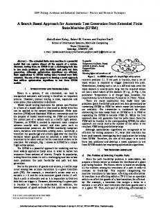
Figure 1. First problem of using one set of cutting planes: (a) theoretical outer loop and (b) low-accuracy outer loop created by one set of cutting planes.

Considering in particular the determination of parting geometry in mold design involving parting line/ curve generation, the slicing approach, compared with other existing approaches, has a significant advantage in that it greatly simplifies this process for free-form models. The root of this advantage stems from the fact that the generation of parting curves for a 3D part is based on the two-dimensional (2D) intersection profiles between the part and multiple cutting planes; however, the use of a single set of cutting planes in conventional slicing methods for 3D models can cause unreasonable results, especially for free-form models with multiple undercuts. It can also be very difficult to achieve a high degree of accuracy, as seen in Figure 1, which shows a hemisphere sliced by one set of cutting planes along the x-axis (Figure 1(a)). The collection of the extreme intersection points between the cutting planes and the hemisphere is shown in Figure 1(b). It is easy to see that the uneven distribution of the extracted intersection points will result in low accuracy of the outer parting curve as well as the inner boundaries of undercuts that are located at specific positions on the hemisphere (u1, u2, and u3). Furthermore, conventional slicing methods use one set of cutting planes to determine the inner loops based on the extraction of extreme points. In most cases, the boundaries of the inner loops are formed by connecting the corresponding left- and right-most intersection points of adjacent loops of adjacent profiles in a certain order. However, this may lead to incorrect results in the case of hemispheres with multiple undercuts. As illustrated in Figure 2(a), the corresponding right- and left-most points (p3ri, p4li) of the two inner loops are actually unsuitable and the resultant inner boundaries are incorrect as shown in Figure 2(b).

Moreover, conventional slicing methods may also need additional criteria to evaluate the results of several alternative choices. Therefore, a new slicing approach using multiple sets of cutting planes for the generation of parting curves of complicated models with free-form surfaces is proposed in this article. This algorithm can overcome all the problems discussed above while also making the process fast and effective. The sets of cutting planes with their individual roles are simultaneously used to create the slicing profiles and to extract the intersection points for all the outer and inner loops of the parting curve. This approach uses tessellated geometry in STL format as the input because STL is a universal CAD exchange format that is widely accepted in various CAD/computer-aided manufacturing (CAM) applications. The parting curves are determined automatically without loss of accuracy, and the algorithm is sufficiently generic to be able to connect with any downstream CAD/ CAM system.

Use of three sets of cutting planes to generate closed loops for a parting curve The main purpose of the proposed slicing algorithm is to determine automatically the best parting curve for a triangulated facet model with a specific parting direction. The algorithm contains the following research issues: selection of the parting direction, formation of cutting planes, extraction of intersection points, collection of points for the outer loop, collection of points for all the inner loops, and construction of closed loops for the parting curve. Figure 3 shows the procedure of the proposed algorithm. Detailed discussion follows.

4

Proc IMechE Part B: J Engineering Manufacture

Figure 2. Second problem of using one set of cutting planes: (a) the right- and left-most points of two inner loops and (b) incorrect inner boundaries.

Figure 3. Procedure of multiple slicing approach for automatic generation of a parting curve.

Selection of a suitable parting direction The best parting direction is usually determined based on the consideration of multiple evaluation criteria such as the projected area, the number of undercuts, and the distance of draw depth. Therefore, one input model may have numerous possible parting directions; however, only a few of these are feasible for use in mold design. In general, a mold designer often chooses one of the principal axes as the desired parting direction. Thus, in this article, the suitable parting direction is selected from among the three principal axes, based on the criterion of maximum rectangular area. By limiting the number of potential parting directions, this selection

process keeps the overall calculation time within an acceptable value. Figure 4 shows a sample model presented in STL format. Coordinates of the vertices of all triangular facets are assessed. The corresponding outermost vertices for the x-, y-, and z-axes are then traced and denoted by the pairs (1, 2), (3, 4), and (5, 6), respectively. Based on these points, the rectangular areas on the x–y, y–z, and z–x principal planes are obtained and used as the criterion to select the suitable parting direction. The z-axis is perpendicular to the maximum rectangular area and is thus chosen as the parting direction.

Lin and Quang

Formation of cutting planes In contrast to the traditional slicing methods that use only one set of cutting planes, the slicing algorithm proposed in this research uses multiple sets. This change helps to avoid problems that arise in determining the boundaries of the inner loops. In this article, the terms ‘‘main,’’‘‘secondary,’’ and ‘‘third’’ set of cutting planes are used to describe the differences in their orientations and roles. Figure 5(a) shows the main set of cutting planes, using the z-axis as the parting direction. The cutting planes of this set are all perpendicular to the xaxis. Each of these cutting planes will be used to find the intersection point pi of the plane with the triangulated facet model. It results in a set of discrete points for each slicing profile. Figure 5(b) illustrates the secondary and third sets of cutting planes. The planes of the secondary set are perpendicular to the y-axis, and

Figure 4. Use of maximum rectangular area to determine the parting direction.

5 the planes of the third set are perpendicular to the zaxis. The role of these two sets of planes is different with that of the main set. For each slicing profile created by a plane of the main set, planes of the secondary and third sets are used as evaluation criteria in order to find suitable points that the parting curve pass through. After the execution of the implement system, the role of three sets of planes will be interchanged. Besides, the slicing distance between two adjacent planes is also decided based on the quality of the facet model. Thus, the tessellated model is scrutinized in the determination of parting curves.

Extraction of intersection points The next step after the formation of cutting planes is to find intersection points between the triangulated facet model and each plane of the main set. To improve the performance and accuracy of the proposed slicing algorithm when using an STL input file, a data filter is introduced to choose and store relevant facets for each cutting plane. This is especially helpful for STL data inputs with a large number of facets; in these cases, the computer memory required for processing all the facets might exceed the available memory, resulting in an unacceptably slow processing speed.35Figure 6(a) illustrates the cutting condition between a plane of the main set and the triangular facets of the STL data generated from the model in Figure 4. The x-coordinate of the cutting plane is used to filter those triangular facets that intersect this plane. Then all the intersection points between the cutting plane and the edges of the filtered facets are computed. One triangular facet may have one or two intersection points with the cutting plane. In Figure 6(a), the triangular facet F1 has one intersection point, p1, with the cutting plane, while the triangular facet F3 has two intersection points, namely, p2 and p3.

Figure 5. (a) Main set of cutting planes. (b) Secondary and third sets of cutting planes.

6


Figure 7. (a) Tentative left- and right-most points in one cutting plane. (b) Four different cases.

Figure 6. (a) Intersection between triangle facets and a plane of the main set. (b) The resultant slicing profile.

In the case of a single intersection point, this point will coincide with one vertex of a triangular facet. Figure 6(b) shows all the intersection points of one slicing profile generated by the intersection of one of the planes of the main set with the triangulated facet model.

Figure 8. (a) Outermost points of one slicing profile. (b) Outermost points of several slicing profiles.

Collection of points for the outer loop A parting curve consists of one outer loop and several inner loops. The outer loop encloses the maximum projected area of the input model along the reverse of the parting direction. Thus, the outer loop is determined by identifying the outermost points on each slicing profile. The main job is to find the left- and right-most points of the intersection of the slicing profile and all cutting planes of the third set. These are the points with maximum and minimum y-values, respectively. Figure 7(a) shows the condition of a tentative left-most point and a tentative right-most point. Because the triangular facets are arbitrarily distributed and each slicing profile is essentially a set of discrete points, one cutting plane of the third set may not detect any intersection point or may determine only one intersection point as the tentative left- or right-most point. Figure 7(b) depicts four different cases of tentative left- and right-most points

in a slicing profile. The final left- and right-most points of a slicing profile are then chosen from the set of tentative left- and right-most points. There should be a single left- and right-most point of a slicing profile. Figure 8(a) shows the two outermost points of one slicing profile, and points (pi1, pi2), (pj1, pj2), and (pk1, pk2) in Figure 8(b) are the outermost points of slicing profiles i, j, and k, respectively. These outermost points are extracted to form the outer loop of the parting curve for the model, as shown in Figure 4. The process to determine the outer loop of a parting curve described above is implemented using one group of plane sets. Figure 9 shows the resulting outer loop formed using the plane sets of Group 1. It is easily observed that the outer loop does not achieve the required level of accuracy. A similar problem can occur when using another group of plane sets, as shown in

Lin and Quang

7

Figure 9. Create an outer loop from plane sets of Group 1.

Figure 10. Create an outer loop from plane sets of Group 2.

Figure 10. The reason for these inaccuracies is the uneven distribution of outermost points determined by plane sets of only one group. To overcome this problem, both groups of plane sets are used in this research to obtain the outer loop of a parting curve. That is, the proposed method uses two groups of plane sets, as listed in Table 1, to alternately slice the triangulated facet model along two main axes, namely, the x- and yaxis. This results in an outer loop that attains the required level of accuracy, as shown in Figure 11. Although the introduction of two groups of plane sets solves the problem of accuracy of the outer loop,

another problem arises. That is the existence of vertical faces on the model. This will lead to many extreme points extracted and the system has difficulty to choose the most suitable one for use as the parting curve. In fact, a molded model may have some or all vertical faces around it. When all around a 3D model are vertical faces, the parting curves must be first determined and the vertical faces are then drafted with respect to the parting curves. This is relatively common in practice of mold design. Depending on the height of vertical faces, the extreme points at the middle or the lowest position are chosen as the suitable points for parting

8


Table 1. Two groups of plane sets. Set of cutting planes

Main set Secondary set Third set

Groups of plane sets Group 1

Group 2

Perpendicular to x-axis Perpendicular to y-axis Perpendicular to z-axis

Perpendicular to y-axis Perpendicular to x-axis Perpendicular to z-axis

Figure 11. Effect of applying two different groups of plane sets.

curves. It is also the choice of the existing methods in order to achieve the flat parting curve/surface that it can be. However, there are rarely cases that only a part of faces of complex models is vertical and it causes the formation of gap in the parting curves. None of researched solutions is proposed for this issue. The gap problem is found similarly in practical design. Although most of the CAD systems provide

their own packages for parting curves design, none of them can fix the gap automatically without any step of manual intervention. Here, the mouse model and Silhouette function of Pro Engineer were used to demonstrate such problem. As shown in Figure 12, using the ‘‘Silhouette’’ function in Pro/Engineer, the outer loop of the parting curve can be found and is illustrated as the ‘‘red curve

Lin and Quang

9

Figure 12. (a) Outer loop containing a small gap. (b) Many right-most intersection points at the gap.

Figure 13. Choosing the outermost point: (a) at the cutting plane k, (b) at the cutting plane k + 1, (c) at all cutting planes, and (d) in 3D view.

PC.’’ There exists a small gap in the parting curve (see ‘‘A small gap’’ in the figure). The checking plane CP is used to cut the model in the vicinity of the gap. It is evident that there are many right-most intersection points (see Figure 12(b)), and Pro/Engineer cannot choose the

most suitable one for use as the parting curve, which causes the formation of a gap. A gap solving method is therefore proposed in this article to find proper curve segments for areas containing gaps. Figure 13 shows the detailed procedure of the

10


method. In the figure, the outermost point on the left is denoted Start and a similar point on the right is denoted End. Cutting plane k of the main set cuts through the model at the first location and results in many right-most intersection points, as shown in Figure 13(a). Among the intersection points with zcoordinates between Start and End, point p1 is closest to Start; thus, p1 is chosen as the most suitable outermost point at that cutting plane. This point then becomes the new Start point for the next cutting plane k + 1 (see Figure 13(b)). In a similar manner, point p2 is chosen as the most suitable outermost point at cutting plane k + 1. This process is repeated until the cutting plane of the main set passes through the End point. The final result is shown in Figure 13(c). In contrast to previous slicing algorithms that use the shortest straight line to connect transitional portions or gap areas, the strategy discussed above forces the transitional segments to lie completely on the outer surfaces, that is, the segments will have the same curvature as the outer surfaces of the input 3D model (see Figure 13(d)).

Collection of points for all inner loops The intersection points of all the inner loops (including undercuts) can be determined based on the concepts of the ‘‘shared vertex’’ and ‘‘adjacent points.’’ Different from the collection of points for the outer loop, the extraction of extreme points based on their coordinates cannot be used here. That is because each intersection profile is only a set of discrete points, hence only two extreme points will be detected there (one in the leftmost and other in the right-most) for parting curves. It will lead to the miss of important points for the inner loops at undercut regions. Even if the proposed system is aware that there are several groups of points in the intersection profile, the extreme points extracted from adjacent groups may not be suitable as illustrated in Figures 2(a) and 2(b). The definition of a shared vertex is described in Figure 14(a). In the figure, pi is an intersection point of the current cutting plane PLi and the edge connecting two vertices Vi1 and Vi2. Similarly, the intersection point pi + 1 is identified between vertices Vi2 and Vi3. Vertex Vi2 thus becomes the common vertex for points pi and pi + 1. The common vertex is then called a shared vertex in this article, and if two intersection points are related by a shared vertex, they are called adjacent points. Figure 14(b) shows two adjacent points related by a shared vertex. Moreover, one intersection point always has two adjacent points on both of its sides. As illustrated in Figure 15, the intersection point pi,1, created by a cutting plane PLi of the main set, has two adjacent points pi,11 and pi,12. The intersection point pi,2 has the same property. Intersection points of the inner loops are collected using cutting planes from the secondary and third sets. The process is implemented by examining the points nearest to the cutting planes and their adjacent points.

Figure 14. (a) Intersection points and corresponding common vertex. (b) Two adjacent points related by a shared vertex.

All intersection points of a slicing profile i in Figure 16 are used to describe the detailed procedure. In Figure 16(a), PL1 is a cutting plane from the secondary set (see Figure 5), and point pi,1 is the nearest point to plane PL1. The points adjacent to pi,1 are pi,11 and pi,12. The y-coordinates of the three related points, namely, pi,1, pi,11, and pi,12, are all larger than the y-coordinate of plane PL1. In other words, these three related points lie on the left side of the cutting plane. Point pi,1 is then classified as a point that belongs to an inner loop. Point pi,2 is the nearest point to cutting plane PL2, and pi,21 and pi,22 are two points adjacent to pi,2. Because points pi,2, pi,21, and pi,22 do not lie on the same side of plane PL2, point pi,2 is not categorized as a point on an inner loop. Figure 16(b) shows the nearest point pi,4 on the right side of cutting plane PL4 and its two adjacent points, pi,41 and pi,42. All points lie on the right side of plane PL4 such that point pi,4 belongs to an inner loop. In contrast, point pi,3 is not classified as a point on an inner loop. Figure 16(c) and (d) shows examples of similar processes with working planes from the third set. In

Lin and Quang

11

Figure 15. Adjacent points.

Figure 16. Points of inner loops collected at (a) the left side, (b) the right side, (c) the top side, and (d) the bottom side of the cutting plane.

these figures, points pi,5 and pi,8 are chosen as points that the inner loops pass through. The process of finding inner-loop points from the entire set of points of a slicing profile is done through all cutting planes of the secondary and third sets, and the results are shown in Figure 17. In Figure 17(a), intersection points pi,1 through pi,6 are collected from a slicing profile and classified as points belonging to the

inner loops. Figure 17(b) shows the intersection points found as inner-loop points at several slicing profiles. Similar to the procedure for determining the outer loop of a parting curve, both Group 1 and Group 2 of the plane sets are alternately used to achieve a high degree of accuracy in generating boundaries of the inner loops (see Table 1 for the definition of planes in these two groups).

12


Figure 18. Two loop points connected by a line segment. Figure 17. Points found as inner-loop points (a) at one slicing profile and (b) at several slicing profiles.

Formulation of closed loops for the parting curve After the extraction of intersection points for the outer loop and inner loops is complete, the next job is to connect associated points by line segments in order to form closed loops. To simplify our discussion, the term ‘‘loop points’’ is used to specify those intersection points that are classified as either the outer loop or the inner loops. The connection between an individual loop point and another loop point can be generated based on the ‘‘shared vertex’’ concept discussed in section ‘‘Collection of points for all inner loops’’—if two loop points are related to a shared vertex, they belong to a loop (the outer loop or one of the inner loops) and can be connected by a line segment. Figure 18 shows an example. In the figure, pi and pj are the two loop points coming from two adjacent slicing profiles. These loop points are related to each other by a common vertex Vk. In this case, Vk is the shared vertex of pi and pj. These two loop points can thus be connected by a straight line to form the boundary of a loop. Two related loop points are connected by a line segment and a closed loop is formed by a series of line segments. In the proposed approach, the slice distance is determined based on the tessellation size (under the file format of STL) and a specified value of cusp height corresponding to the quality of the tessellated model. The concept of maximum allowable cusp height Cmax was successfully attempted and widely accepted by many researchers and practical systems.36–39 According to their approaches, those distances that do not satisfy the cusp height requirement (c \ Cmax) will be further subdivided into smaller distances. This will ensure the

successful search of ‘‘shared vertex’’ and the connection of ‘‘loop points’’ for the parting curves. In order to form a closed loop, each individual loop point must be connected to two other related points on both of its sides. Figure 19 illustrates a typical instance. In Figure 19(a), which shows a top view of the facet model, cutting planes i, i + 1, and i + 2 intersect the model and result in loop points pi,1, (pi + 1,1, pi + 1,2), and (pi + 2,1, pi + 2,2), respectively. The loop point pi,1 is connected to two related points, pi + 1,1 and pi + 1,2, based on the relationship with the shared vertex Vi of the triangular facet, while the loop point pi + 1,1 is connected to two other related points, pi,1 and pi + 2,1, through the corresponding shared vertices Vi and Vi + 1,1. Similar conditions hold for loop points pi,1, pi + 1,2, pi + 2,2, and others. These loop points are then connected by line segments to form closed loops. Figure 19(b) shows the final closed loops.

System implementation The proposed methodology has been implemented using a commercial software package—MATLAB 9.0. First, the STL data of test models were generated and checked for validity. The parting curves were generated based on the procedure and methods discussed above. The STL data were also used in Pro/Engineer Wildfire 5.0 as an input model, and the function Silhouette in Pro/Engineer was used to create a parting curve. The results from our system and from Pro/Engineer are then compared. Several case studies are presented below.

Case study 1 Figure 20(a) shows a mouse model used to test the implemented system. The model contains many

Lin and Quang

13

Figure 19. (a) Line segments connecting corresponding loop points. (b) Closed loops formed by a series of line segments.

Figure 20. Case study 1: (a) part model, (b) STL data, (c) parting curve found by our implemented system, and (d) parting curve generated by Pro/Engineer.

free-form surfaces and some of them have vertical regions (a vertical region means that only a small part of face/surface is vertical). This is the reason that causes the gap problem when determining the outer parting curves for the model as mentioned in section ‘‘Collection of points for the outer loop.’’ The gap is also illustrated in Figure 20(d) when the outer parting curve of the mouse model is found by the Silhouette function of Pro/Engineer. For this situation, the z-axis

was chosen as the primary parting direction and the facet model in STL format is shown in Figure 20(b). Using the proposed gap solving method, the implemented system successfully generates a closed parting curve without any existence of gap, as illustrated in Figure 20(c). The parting curve is thus better than the one generated using the Silhouette function in Pro/Engineer and it is ready for further creating parting surfaces and splitting the mold pieces.

14


Figure 21. Case study 2: (a) part model, (b) STL data, (c) parting curve found by our implemented system, and (d) parting curve generated by Pro/Engineer.

Case study 2 The second model used to test the implemented system was a hemisphere with multiple undercuts (Figure 21(a)). This input model was chosen because it includes a surface with large curvature and many undercuts distributed along the periphery. Similar to Case study 1, the vertical direction was selected to be the primary parting direction (z-axis). The STL file input and the resultant parting curve are presented in Figure 21(b) and (c), respectively. By comparing the parting curve generated by the implemented system with that generated by the Silhouette function in Pro/Engineer (Figure 21(d)), it can be seen that there is a large difference between the two. In the curve generated by the Silhouette feature, the boundaries of the undercut in Figure 21(d) are not fully closed, and the mold designers must use additional functions to modify them into closed loops. In contrast, the parting curve in Figure 21(c), which was generated by our implemented system, does not present this problem. Although there are many undercuts with a variety of different undercut

directions, the implemented system still accurately determines their boundaries. The generated parting curve can be used directly to obtain parting surfaces for future mold design.

Case study 3 The plastic cover shown in Figure 22 was used to further evaluate the performance of the implemented system. The geometric characteristics of this model could be adjusted to create different conditions for the generation of parting curves. First, all vertical surfaces were drafted (see Figure 22(a)), and the corresponding STL data are presented in Figure 22(b). The primary parting direction was selected to be the z-axis. The parting curve obtained by our implemented system contains an outer loop and several inner loops, as shown in Figure 22(c). Compared with the result from Pro/Engineer (Figure 22(d)), it is easily observed that the two results are the same. They both represent the most reasonable option among several possible choices of parting curves

Lin and Quang

15

Figure 22. Case study 3: (a) part model having draft angles at all outer surfaces, (b) STL data, (c) parting curve found by our implemented system, and (d) parting curve generated by Pro/Engineer.

Figure 23. Case study 3 (the model having draft angle for only back side of the outer surface): (a) parting curve generated by Pro/ Engineer and (b) parting curve found by our implemented system.

because they fully represent the important features of the input model. Next, instead of using draft angles for all vertical surfaces, the model was changed to leave a draft angle for only the back surface. Figure 23(a) shows the parting curve found using Pro/Engineer in which some important features are not represented (see features inside the blue circle). Figure 23(b) shows the correct results as generated by our implemented system. For efficient implementation of the proposed algorithm, a filtered program was employed to prune unnecessary information from the STL data. Through the running example—the hemisphere model used to

present the capacity of the algorithms, that is, Case study 2, the computation time was acceptable although it was not a simple part (there are multiple undercuts distributed along the periphery of the model). It generated all the outer and inner loops of parting curves within 4 min. The proposed system also takes 1 min and 48 s to handle the mouse model (Case study 1) and over 3 min for the plastic cover (Case study 3).

Conclusion The multi-slicing approach presented in this article is an innovative method for handling 3D models with

16 free-form surfaces. As described in the methodology section and case studies, the proposed algorithm presents two significant improvements that can overcome the problems encountered in the existing methods found in the literature. First, using three sets of slicing planes simultaneously and flexibly, the approach can automatically recognize both the closed outer loop and some inner loops of parting curves for complex CAD models. Second, different from conventional STL slicing algorithms, which require storing the intersection points together with the line vectors to obtain the slice contours, the proposed slicing algorithm stores only the intersection points in order to detect the boundaries of intrinsic geometric features. This feature is certainly very helpful in handling large facet data, and thus, the computational complexity will be significantly improved. Although there exist some limitations, mainly from the poor quality of the input tessellation data of the molded parts, which might cause several unwanted segments of parting curves, we expect that the algorithms described in this article will provide the foundations for automating the generation of parting curves. For more convenient use with current CAD/CAM systems and applications in industry, the research of increasing the quality of triangle facets should be addressed in the future work. Declaration of conflicting interests The authors declare that there is no conflict of interest. Funding This research received no specific grant from any funding agency in the public, commercial, or not-for-profit sectors. References 1. Ravi B and Srinivasan MN. Decision criteria for computer-aided parting surface design. Comput Aided Design 1990; 22(1): 11–18. 2. Fu MW, Fuh JYH and Nee AYC. Undercut feature recognition in an injection mould design system. Comput Aided Design 1999; 31(12): 777–790. 3. Ye XG, Fuh JYH and Lee KS. A hybrid method for recognition of undercut features from moulded parts. Comput Aided Design 2001; 33(14): 1023–1034. 4. Lu HY and Lee WB. Detection of interference elements and release directions in die-cast and injection-moulded components. Proc IMechE, Part B: J Engineering Manufacture 2000; 214(6): 431–441. 5. Ismail N, Bakar NA and Juri AH. Recognition of cylindrical-based features using edge boundary technique for integrated manufacturing. Robot Cim: Int Manuf 2004; 20(5): 417–422. 6. Khardekar R, Burton G and McMains S. Finding feasible mold parting directions using graphics hardware. Comput Aided Design 2006; 38(4): 327–341.

Proc IMechE Part B: J Engineering Manufacture 7. Chen LL, Chou SY and Woo TC. Partial visibility for selecting a parting direction in mould and die design. J Manuf Syst 1995; 14(5): 319–330. 8. Fu MW, Fuh JYH and Nee AYC. Generation of optimal parting direction based on undercut features in injection molded parts. IIE Trans 1999; 31(10): 947–955. 9. Nee AYC, Fu MW, Fuh JYH, et al. Determination of optimal parting direction in plastic injection mold design. CIRP Ann: Manuf Techn 1997; 46(1): 429–432. 10. Chen YH, Wang YZ and Leung TM. An investigation of parting direction based on dexel and fuzzy decision making. Int J Prod Res 2000; 38(6): 1357–1375. 11. Dhaliwal S, Gupta SK, Huang J, et al. Algorithms for computing global accessibility cones. J Comput Inf Sci Eng 2003; 3(3): 200–209. 12. Ravi B and Srinivasan MN. Computer-aided parting surface generation. In: Proceedings of ASME manufacturing international conference, Atlanta, GA, 25–28 March 1990, pp.125–129. New York, NY: The American Society of Mechanical Engineers. 13. Tan ST, Yuen MF, Sze WS, et al. Parting lines and parting surfaces of injection molded parts. Proc IMechE, Part B: J Engineering Manufacture 1990; 204: 211–221. 14. Weinstein M and Manoochehri S. Geometric influence of a molded part on the draw direction range and parting curve locations. J Mech Design 1996; 118(1): 29–39. 15. Weinstein M and Manoochehri S. Optimum parting line design of molded and cast parts for manufacturability. J Manuf Syst 1997; 16(2): 1–12. 16. Nee AYC, Fu MW, Fuh JYH, et al. Automatic determination of 3-D parting lines and surfaces in plastic injection mould design. CIRP Ann: Manuf Techn 1998; 47(1): 95–108. 17. Fu MW, Nee AYC and Fuh JYH. The application of surface visibility and moldability to parting line generation. Comput Aided Design 2002; 34(6): 469–480. 18. Wong T, Tan ST and Sze WS. Parting line formation by slicing a 3D CAD model. Eng Comput 1998; 14(4): 330–343. 19. Paramio MAR, Garcia JMP, Chueco JR, et al. A procedure for plastic parts demoldability analysis. Robot Cim: Int Manuf 2006; 22(1): 81–92. 20. Serrar M and Gabriele GA. Automatic generation of parting surfaces and mold halves. In: Proceedings of the computers in engineering conference and the engineering database symposium, ASME, Boston, MA, 17–20 September 1995, pp.75–82. New York, NY: The American Society of Mechanical Engineers. 21. Fu MW, Nee AYC and Fuh JYH. Core and cavity generation method in injection mould design. Int J Prod Res 2001; 39(1): 121–138. 22. Li CL. Automatic parting surface determination for plastic injection mould. Int J Prod Res 2003; 41(15): 3529–3547. 23. Li CL, Yu KM and Li CG. A new approach to parting surface design for plastic injection moulds using the subdivision method. Int J Prod Res 2005; 43(3): 537–561. 24. Shin KH and Lee KW. Design of side cores of injection molds from automatic detection of interference faces. J Des Manuf 1993; 3: 225–236. 25. Ye XG, Fuh JYH and Lee KS. Automatic undercut feature recognition for side core design of injection molds. J Mech Design 2004; 126(3): 519–526.

Lin and Quang 26. Banerjee AG and Gupta SK. Geometrical algorithms for automated design of side actions in injection moulding of complex parts. Comput Aided Design 2007; 39(10): 882–897. 27. Fuh JYH, Wu SH and Lee KS. Development of a semiautomated die casting die design system. Proc IMechE, Part B: J Engineering Manufacture 2002; 216: 1575–1588. 28. Fu MW. The application of surface demoldability and moldability to side-core design in die and mold CAD. Comput Aided Design 2008; 40(5): 567–575. 29. Ran JQ and Fu MW. Design of internal pins in injection mold CAD via the automatic recognition of undercut features. Comput Aided Design 2010; 42(7): 582–597. 30. Zhou H, Zhang Y, Wen J, et al. Mould cooling simulation for injection moulding using a fast boundary element method approach. Proc IMechE, Part B: J Engineering Manufacture 2010; 224: 653–662. 31. Elyasi M, Bakhshi-Jooybari M, Gorji A, et al. New die design for improvement of die corner filling in hydroforming of cylindrical stepped tubes. Proc IMechE, Part B: J Engineering Manufacture 2009; 223: 821–827. 32. Singh R, Madan J and Kumar R. Automated identification of complex undercut features for side-core design for

17

33.

34.

35.

36.

37.

38.

39.

die-casting parts. Proc IMechE, Part B: J Engineering Manufacture 2014; 228(9): 1138–1152. Bidkar RA and McAdams DA. Methods for automated manufacturability analysis of injection-molded and diecast parts. Res Eng Des 2010; 21(1): 1–24. Denkena B, Schurmeyer J, Bos V, et al. CAD-based cost calculation of mould cavities. Prod Engineer 2011; 5(1): 73–79. Choi SH and Kwok KT. A memory efficient slicing algorithm for large STL files. In: Proceedings of solid freeform fabrication symposium, Austin, TX, 9–11 August 1999, pp.155–162. Austin, TX: University of Texas. Dolenc A and Makela I. Slicing procedures for layered manufacturing techniques. Comput Aided Design 1994; 26(2): 119–126. Cormier D, Unnanon K and Sanni E. Specifying nonuniform cusp height as a potential for adaptive slicing. Rapid Prototyping J 2000; 6(3): 204–211. Sabourin E, Houser SA and Bohn JH. Adaptive slicing using stepwise uniform refinement. Rapid Prototyping J 1996; 2(4): 20–26. Tata K, Fadel G, Bagchi A, et al. Efficient slicing for layered manufacturing. Rapid Prototyping J 1998; 4(4): 151–167.