AbstractâIn this letter, we aim to present a near-maximum- likelihood (ML) decoding algorithm with low-complexity for wider ranges of SNR and system ...
IEEE TRANSACTIONS ON WIRELESS COMMUNICATIONS, VOL. 11, NO. 1, JANUARY 2012
33
A Near-ML Decoding with Improved Complexity over Wider Ranges of SNR and System Dimension in MIMO Systems Junil Ahn, Student Member, IEEE, Heung-No Lee, Member, IEEE, and Kiseon Kim, Senior Member, IEEE Abstract—In this letter, we aim to present a near-maximumlikelihood (ML) decoding algorithm with low-complexity for wider ranges of SNR and system dimension in multiple-inputmultiple-output (MIMO) systems. Based on the proposed radius design criterion, we introduce the effective radius (ER) which is determined using the statistics of path metric under correct and incorrect decoding cases. Since the constraint established by the ER maintains tightness during most search procedure, the proposed scheme further improves the complexity, and its performance loss is still negligible by properly selecting design probabilities. Index Terms—Multiple-input-multiple-output (MIMO) detection, sphere decoding (SD), near-maximum-likelihood decoding, lattice decoding.
I. I NTRODUCTION
S
PHERE-DECODING (SD) [1]–[3] has attracted substantial attention because of its maximum-likelihood (ML) performance with low average complexity for multiple-inputmultiple-output (MIMO) detection [4]. The basic premise of SD is that it finds the closest point to a given point within the hypersphere of a certain radius. The SD search procedure is interpreted as a depth-first tree search (DFTS) over a tree with as many layers as the number of transmit antennas. Recently, several statistical pruning approaches (SPAs) have been proposed based on a DFTS in attempts to further alleviate the SD complexity at the expense of minimal performance loss [5]–[7]. The principle of SPAs lies on the usage of a predefined radius (PR) or a reduced dynamic update radius (DUR) derived statistically to prune branches leading to incorrect solutions at a high probability. However, existing strategies are efficient only in certain SNRs and system dimensions (i.e., the number of transmit antennas), or have algorithmic drawbacks as follows: 1) Increasing radii algorithm (IRA) [5] has computational benefits only for high SNRs and large dimensional systems. 2) Probabilistic tree pruning SD (PTPSD) [6] is efficient only for low-to-mid SNRs and moderate size systems. 3) Inter-search radius control (ISRC) [7] adjusts the radius only when a solution is found at the last depth, and the proper selection of design probabilities for arbitrary system configurations is yet somewhat vague. Motivated by the observation that above issues can be resolved by a proper design, we propose a strategy based on a DFTS to perform a low-complexity near-ML decoding over wider ranges of SNR and system dimension. To fulfil the
Manuscript received March 15, 2011; revised August 24, 2011; accepted October 4, 2011. The associate editor coordinating the review of this letter and approving it for publication was A. Chockalingam. This work was supported by the International Joint R&D Program funded by the Ministry of Knowledge Economy (MKE, Korea), and partially by National Research Foundation of Korea (NRF) (No. 2011-0027682). The authors are with the School of Information and Mechatronics (SIM), Gwangju Institute of Science and Technology (GIST), Gwangju, Republic of Korea (e-mail: {jun, heungno, kskim}@gist.ac.kr). Digital Object Identifier 10.1109/TWC.2011.110811.110471
proper design, we establish a radius design criterion for lowcomplexity decoding and then introduce the effective radius (ER) which is obtained using the statistics of path metric under correct and incorrect decoding cases. Also, we present a strategy to select design probabilities supporting a near-ML performance. The upper bound on the expected complexity is analyzed to verify the complexity reduction effect. Note that the proposed scheme pursues further reduction of the average complexity, like efforts in [3], [5]–[7]. However, the actual complexity of DFTS based methods is variable, and the worst-case complexity sometimes leads to throughput latency for hardware implementation. Thus, the worst-case complexity of the proposed scheme is also evaluated and compared to that of the fixed-complexity SD (FSD) [8] which performs decoding in a fixed number of operations. For reference, local neighborhood search algorithms, termed as likelihood ascent search (LAS) [9] and reactive tabu search (RTS) [10] have been proposed for very large MIMO detection. However, these algorithms have relatively improved complexity only for systems with quite large dimensions (e.g., hundreds real dimensions) and are also not in the framework of tree search approaches. Thus, algorithm comparisons are limited to SD and its variants in this letter. II. S YSTEM M ODEL AND S PHERE D ECODING As in [3], [6], an equivalent real-valued MIMO linear model is given by y = H¯ x + z, (1) where y ∈ ℛ𝑁 is a received real vector, x ¯ ∈ 𝒜𝑀 is a transmitted vector, x ¯ is independently drawn from an 𝑀 -dimensional { } 𝐿−3 𝐿−3 𝐿−1 𝑀 𝐿-PAM constellation 𝒜𝑀 = − 𝐿−1 , 2 , − 2 , ..., 2 , 2 z is an additive noise vector, and the entries of z follow an independent and identically distributed ( ) (i.i.d.) zero-mean Gaussian distribution, i.e., 𝑧𝑖 ∼ 𝒩 0, 𝜎𝑧2 . H ∈ ℛ𝑁 ×𝑀 is a column full rank real matrix with 𝑁 ≥ 𝑀 , and ) ( channel the entries of H ∼ 𝒩 0, 𝜎ℎ2 . 𝐸𝑠 is the total transmit energy in each channel use such that the SNR per receive antenna is defined as SNR = (𝐸𝑠 𝜎ℎ2 )/𝜎𝑧2 . We let 𝑁 = 𝑀 for H henceforth for the sake of simplicity. Note that 𝑛𝑇 × 𝑛𝑅 MIMO system with 𝐿2 -QAM corresponds to 𝑀 × 𝑁 realvalued model with 𝐿-PAM, where 𝑛𝑇 and 𝑛𝑅 are the number of transmit and receive antennas, respectively, and 2𝑛𝑇 = 𝑀 and 2𝑛𝑅 = 𝑁 . SD searches over candidate vectors x such that x − x)∥2 ≤ 𝑑2 , ∥y − Hx∥2 = ∥R(ˆ
(2)
where 𝑑 is a DUR, H = QR from QR decomposition of H, Q is a unitary matrix, R is an upper triangular matrix with non-negative diagonal entries, and x ˆ = R−1 Q𝑇 y. If 𝑑2 is large enough to include any one x, SD guarantees to provide an ML solution x ˆML having the minimum metric.
c 2012 IEEE 1536-1276/12$31.00 ⃝
34
IEEE TRANSACTIONS ON WIRELESS COMMUNICATIONS, VOL. 11, NO. 1, JANUARY 2012
Because of the triangularity of R in (2), one can construct a tree of depth 𝑀 , which is indexed from depth (or dimension) 𝑘 = 1 to 𝑀 . In this tree, branches at depth 𝑘 correspond to candidate symbols 𝑥𝑀−𝑘+1 , and thus paths from depth 1 to 𝑀 are regarded as candidate vectors x. By denoting w = R(ˆ x − x), a ∑ path metric from depth 𝑘 (𝑘) 1 to 𝑘 is given by 𝑃𝑘 (x(𝑘) ) = = 𝑖=1 𝐵𝑖 , where x 2 𝑇 [𝑥𝑀−𝑘+1 , 𝑥𝑀−𝑘+2 , ..., 𝑥𝑀 ] , and 𝐵𝑖 = ∣𝑤𝑀−𝑖+1 ∣ is a branch metric at depth 𝑖. Due to the casuality of DFTS, SD searches only x(𝑘) satisfying the following constraint condition at each depth 𝑘: 𝑃𝑘 (x(𝑘) ) ≤ 𝑑2 for 𝑘 = 1, 2, ..., 𝑀.
(3)
Whenever an x satisfying (3) is found at the last depth 𝑀 , 𝑑2 is updated with the full path metric 𝑃𝑀 (x) of the found x, thereby reducing 𝑑2 from previous value. This search procedure continues until only one x remains within the search ˆML space specified by 𝑑2 , at which time x is the ML solution x under the condition of (2). There are two enumeration methods in order to sort candidate symbols to be searched at each depth 𝑘: Fincke-Pohst (FP) [1] and Schnorr-Euchner (SE) [2] strategies. In FP enumeration, candidates are spanned following the lexicographic order, whereas SE enumeration examines candidates in the ascending order of their metrics; resulting in a much faster search. III. P ROPOSED D ECODING A LGORITHM In this section, we will introduce existing SPAs and then explain a new decoding algorithm. A. Existing Statistical Pruning Approaches (SPAs) According to the usage of radius, SPAs can be classified as the PR based strategy (i.e., IRA) and the DUR based one (i.e., PTP-SD and ISRC). IRA is based on FP enumeration, and it uses an increasing sequence of PRs as 𝑟𝑘2 = (𝛿(𝜖) log 𝑀 +𝑘)𝜎𝑧2 [5], where 𝛿(𝜖) is a scaling parameter. The computation of 𝛿(𝜖) involves numerically solving a highly underdetermined equation system, given by ([5], 14). Thus, the values of 𝛿(𝜖) for some configurations were listed in Table V of [5]. PTP-SD employs SE strategy and uses the reduced DUR obtained by subtracting a pure noise contribution. ISRC was then proposed to further reduce the PTP-SD complexity via an additional radius control. Because this radius control is performed only when x is found at the last depth 𝑀 , the constraint condition of ISRC is rather loose in initial depths. B. Radius Design Criterion for Low-Complexity Decoding The complexity of tree search algorithms including SD and SPAs heavily depends on the choice of radius. Thus, we establish a radius design criterion to perform low-complexity decoding over wider ranges of SNR and system dimension. To do this, the followings are discussed. First, the DUR is computationally efficient in low SNRs, whereas the PR is more preferable in high SNRs. In SE enumeration based SD (i.e., SESD), the initial value of DUR is set to be very large such as infinity [3]. Then, the path metric of the first found vector x ˆB is referred to as the Babai metric,
xB ∥2 [3]. Let 𝑃ML = ∥z∥2 which is given by 𝑃B = ∥y − Hˆ be the ML metric, which is proportional to noise variance 𝜎𝑧2 , i.e., 𝑃ML ∝ 𝜎𝑧2 . The path metric difference ∣𝑃B − 𝑃ML ∣ would be small in low SNRs since both 𝑃B and 𝑃ML prominently depend on the noise in those SNRs. However, as SNR increases, the situation that 𝑃B ≫ 𝑃ML is dominant [3] because 𝑃ML is quite small in high SNRs; ∣𝑃B −𝑃ML ∣ would increase, and thus there exist many candidates to be examined between x ˆB and x ˆML . On the other hand, since the PR is generally designed to be proportional to the noise variance, it has a smaller radius value as SNR increases. Hence, the PR is more promising in high SNRs in the sense of complexity. Secondly, as the dimension 𝑀 increases, a strategy using different radius per each depth becomes more computationally efficient than a scheme with a single radius over the whole depth. Since the conventional SD employs a large 𝑑 over the entire is expressed as 𝐶SD = ∑𝑀 search2 space, the SD complexity 2 𝐶 (𝑑 ), where 𝐶 (𝑑 ) is the complexity from depth 𝑘 𝑘=1 𝑘 𝑘, and 𝐶𝑘 (𝑑2 ) ∝ 𝑑. Assuming that the usage of radius 𝑑𝑘 per depth 𝑘 such that 𝑑 ≥ 𝑑𝑘 , the total complexity decreases because 𝐶𝑘 (𝑑2 ) ≥ 𝐶𝑘 (𝑑2𝑘 ). Here,(we define the complexity ) ∑𝑀 2 2 decrement as 𝐶𝐷(𝑀 ) = 𝑘=1 𝐶𝑘 (𝑑 ) − 𝐶𝑘 (𝑑𝑘 ) . Since 𝐶𝐷(𝑀 ) ∝ 𝑀 , the computational efficiency of the strategy using different radius per depth grows as 𝑀 increases. From the above discussions, we establish a radius design criterion for low-complexity decoding as follows: Adaptive employment of PR and DUR, and the usage of different radius per each depth such that 𝑑𝑘+1 ≥ 𝑑𝑘 . C. Proposed Effective Radius (ER) To support the aforementioned design criterion, we propose the effective radius (ER) 𝑑˜𝑘 using a new PR 𝑑′𝑘 and a refined DUR 𝑑¯𝑘 , where these radii are determined based on the statistics of path metric under correct and incorrect decoding cases, respectively (this issue will be discussed later in detail). Then, we determine 𝑑˜2𝑘 as ¯2 𝑑˜2𝑘 = min(𝑑′2 𝑘 , 𝑑𝑘 ) for 𝑘 = 1, 2, ..., 𝑀.
(4)
Since the PR and the DUR depend on the noise statistics and the full path metric 𝑃𝑀 (x) found at the last depth 𝑀 , respectively, they might be effective at different search time and depth. Thus, as seen in (4), the taking the minimum ¯2 between 𝑑′2 𝑘 and 𝑑𝑘 can be an adaptive application of both radii to compensate for each other’s weakness. In addition, since the PR 𝑑′𝑘 will be determined such that 𝑑′𝑘+1 ≥ 𝑑′𝑘 , the ER 𝑑˜𝑘 is also in the ascending manner. Thus, the above radius design criterion is satisfied. Note that contrary to ISRC, the ER 𝑑˜𝑘 is adjusted at all depths; thus, aggressive tree pruning is accelerated from early search time and depths. Now, we will exploit the probabilistic perspective of the path metric to determine 𝑑′𝑘 and 𝑑¯𝑘 . From (1) and (2), w can be rewritten as w = R(¯ x − x) + Q𝑇 z, and then from the (𝑘) definition of 𝑃𝑘 (x ), we have �2 � �2 � � � � � x(𝑘) − x(𝑘) ) + z(𝑘) � , (5) 𝑃𝑘 (x(𝑘) ) = �w(𝑘) � = �H(𝑘) (¯ where H(𝑘) is a certain matrix such that H(𝑘) = Q(𝑘) R(𝑘) from its QR decomposition, R(𝑘) is a 𝑘 × 𝑘 lower right submatrix of R, and Q(𝑘) is the corresponding unitary submatrix [11]. Since in (5), the elements of H(𝑘)
AHN et al.: A NEAR-ML DECODING WITH IMPROVED COMPLEXITY OVER WIDER RANGES OF SNR AND SYSTEM DIMENSION IN MIMO SYSTEMS
) ( follow 𝒩 0,( 𝜎ℎ2 , intuition tells us )that the entries of w(𝑘) 𝒩 0, 𝜎ℎ2 ∥¯ x(𝑘) − )x(𝑘) ∥2 + 𝜎𝑧2 ; thus, 𝑃𝑘 (x(𝑘) ) ∼ ( 2∼ (𝑘) 2 (𝑘) 2 𝜒𝑘 𝜎ℎ ∥¯ x − x ∥ + 𝜎𝑧2 , where 𝜒2𝑘 (𝜎 2 ) is a Chi-square distribution with 𝑘 degrees of freedom, and its probability (𝑘/2)−1 −𝑥/(2𝜎2 ) 𝑒 density function (PDF) is 𝑥 2𝑘/2 Γ(𝑘/2)𝜎 in which Γ(𝑘) 𝑘 denotes the Gamma function. ( ) that 𝜂𝑃𝑘 (x(𝑘) ) ∼ 𝜒)2𝑘 𝜎𝑧2 ∙ Determination of PR 𝑑′𝑘 : Note ( x(𝑘) − x(𝑘) ∥2 + 𝜎𝑧2 ≤ 1, for any x(𝑘) , where 𝜂 = 𝜎𝑧2 / 𝜎ℎ2 ∥¯ and the equality holds if and only if a correct decoding ¯ (𝑘) ; thus, 𝑃𝑘 (x(𝑘) ) ≥ performs until depth 𝑘, i.e., x(𝑘) = x (𝑘) ¯ ). 𝑃𝑘 (¯ x ), except for the case of ML error (i.e., x ˆML ∕= x Accordingly, the usage of statistics of 𝑃𝑘 (¯ x(𝑘) ) is reasonable to obtain a tight PR. Hence,( the squared PR)𝑑′2 𝑘 is achieved at = 1 − 𝛼, where each depth 𝑘 such that Pr 𝑃𝑘 (¯ x(𝑘) ) ≤ 𝑑′2 𝑘 𝛼 is the design probability. Then, 𝑑′2 𝑘 is given by −1 𝑑′2 (1 − 𝛼; 𝑘)𝜎𝑧2 for 𝑘 = 1, 2, ..., 𝑀, 𝑘 = 𝐹
(6)
where 𝐹 −1 (𝑥; 𝑘) is the inverse cumulative distribution function (CDF) of 𝜒2𝑘 (1), 𝐹 (𝑥; 𝑘) = 𝛾(𝑥/2, 𝑘/2) is the CDF of ∫ 𝑥 𝑘−1 𝜒2𝑘 (1), and 𝛾(𝑥, 𝑘) = 0 𝜆Γ(𝑘) 𝑒−𝜆 𝑑𝜆 is the regularized gamma function. Note that from (6), we know that 𝑑′𝑘+1 ≥ 𝑑′𝑘 for all 𝑘. ∙ Determination of refined DUR 𝑑¯𝑘 : The direct application of DUR 𝑑 is inadequate especially in early search time and depth since one initially sets to 𝑑 = ∞. Thus, instead of 𝑑2 , we employ the refined DUR square as 𝑑¯2𝑘 = 𝑑2 − 𝑢𝑘 , where 𝑢𝑘 is the expected metric of unvisited depths (EMU) at depth 𝑘. In order to determine 𝑢𝑘 , we adopt the statistics of path metric under one neighbor decoding error, where a candidate 𝑥𝑖 is selected as a neighbor closest to the transmitted 𝑥 ¯𝑖 at one certain unvisited depth. Under the hypothesis of this decoding error, the metric contributed from unvisited depths (from depth 𝑘 + 1 to 𝑀 ) (at current depth 𝑘, denoted as 𝑈𝑘 , satisfies that ) 2 2 , where 𝜎𝑠𝑢𝑚 = 𝜎ℎ2 + 𝜎𝑧2 . Then, the EMU 𝑈𝑘 ∼ 𝜒2𝑀−𝑘 𝜎𝑠𝑢𝑚 at depth 𝑘, i.e., 𝑢𝑘 is obtained such that Pr(𝑈𝑘 ≤ 𝑢𝑘 ) = 𝛽, where 𝛽 is also one of the design probabilities. Thus, 𝑢𝑘 is given by 2 for 𝑘 = 1, 2, ..., 𝑀 − 1. 𝑢𝑘 = 𝐹 −1 (𝛽; 𝑀 − 𝑘)𝜎𝑠𝑢𝑚
(7)
Basically, a large 𝑢𝑘 is favourable in terms of complexity. In [6], the perfect decoding is supposed to assess the metric from the unvisited depths. However, in high SNRs, this strategy produces a quite small value; thus its complexity reduction becomes negligible in those SNRs. As a result, the proposed scheme performs a DFTS by using the following condition established by the ER 𝑑˜𝑘 : 𝑃𝑘 (x(𝑘) ) ≤ 𝑑˜2𝑘 for 𝑘 = 1, 2, ..., 𝑀.
(8)
Compared to the condition of (3), the constraint of (8) can further maintain tightness during most search procedure because of the above elaborate radius design for the ER 𝑑˜𝑘 . D. Design Probabilities for Near-ML Performance The decoding performance depends on the design probabilities 𝛼 and 𝛽. Basically, in (6) and (7), quite large 𝛼 and 𝛽 would incur performance loss or decoding failure, although it has a trade-off between complexity and performance. Thus, we have to carefully select 𝛼 and 𝛽 to ensure the nearML performance. Here, 𝛼 is scheduled in an exponentially
35
deceasing manner such as {0.1, 0.01, 0.001, ...}, like the approach in [5]. This sequence of small probabilities is helpful to mitigate performance degradation. Also, this way would be beneficial for alleviating the complexity incurred by algorithm restarting since it makes decoding succeed mostly in initial probabilities (e.g., 0.1 or 0.01). On the other hand, 𝛽 is selected as {𝜀, 𝜀, 𝜀, ...}, where 0 ≤ 𝜀 ≪ 1. One decides 𝜀 according to a target error probability (e.g., 0.001). Note that the proposed algorithm starts with 𝛼 = 0.1 and 𝛽 = 𝜀, and if any x is not found, then the next search trial is executed with subsequent probabilities. This continues until decoding success is achieved. In ISRC, one should consider the behavior of the full path metric 𝑃𝑀 (x) to find the design probabilities providing a good trade-off. However, this probability selection is rather difficult to be done without several empirical results for different SNRs and system sizes. IV. E XPECTED C OMPLEXITY A NALYSIS The actual complexity of DFTS based decoding strategies is a random variable depending on the channel and the noises that have known distributions, and the complexity in a worst case sense tends to be exponential. In this case, it is useful to examine the expected complexity and select it as a practical measure in order to assess algorithmic complexity. Also, the complexity analysis for decoding algorithms is required to analytically verify the reduction effect in complexity and estimate the complexity behavior [11], [12]. For the above reasons, we derive the upper bound on the expected (or averaged) complexity of the proposed scheme (and evaluate mainly the average complexity in the next simulation results). Our analysis is done under the assumption of FP enumeration via the framework of [11]. The expected complexity of the proposed scheme is defined as 𝐶=
𝑀 ∑
𝐸𝑝 (𝒟𝑘 )𝑓(𝑘),
(9)
𝑘=1
where 𝐸𝑝 (𝒟𝑘 ) is the expected number of points included in 𝒟𝑘 , 𝒟𝑘 denotes the search space including all points that satisfy the condition of (8) from depth 1 to 𝑘, and 𝑓 (𝑘) is the number of floating point operations (FLOPs) required to search for each point at depth 𝑘, which is 2𝑘 + 11 + 2𝐿 since our strategy requires an additional subtraction for 𝑑¯2𝑘 and one comparison for 𝑑˜2𝑘 of (4), compared to that of SD, i.e., 𝑓SD = 2𝑘 + 9 + 2𝐿 [11]. From the definition of 𝒟𝑘 , Pr(x(𝑘) ∈ 𝒟𝑘 ) = Pr(𝑃1 (x(1) ) ≤ 𝑑˜21 , 𝑃2 (x(2) ) ≤ 𝑑˜22 , ..., 𝑃𝑘 (x(𝑘) ) ≤ 𝑑˜2𝑘 ) ≤ Pr(𝑃𝑘 (x(𝑘) ) ≤ 𝑑˜2𝑘 ). Thus, we have ∑ ∑ Pr(x(𝑘) ∈ 𝒟𝑘 ) ≤ Pr(𝑃𝑘 (x(𝑘) ) ≤ 𝑑˜2𝑘 ). 𝐸𝑝 (𝒟𝑘 ) = x(𝑘)
x(𝑘)
(10) ( ) Since 𝑃𝑘 (x(𝑘) ) ∼ 𝜒2𝑘 𝜎ℎ2 ∥¯ x(𝑘) − x(𝑘) ∥2 + 𝜎𝑧2 , the right term of (10) is rewritten as ) ( ∑ ∑ 𝑘 𝑑˜2𝑘 (𝑘) 2 ˜ , , Pr(𝑃𝑘 (x ) ≤ 𝑑𝑘 ) = 𝑛𝑘 (𝑞)𝛾 2(𝜎𝑧2 + 𝜎ℎ2 𝑞) 2 𝑞 x(𝑘) (11) where 𝑛𝑘 (𝑞) is the number of pairs (¯ x(𝑘) , x(𝑘) ) such that ∥¯ x(𝑘) − x(𝑘) ∥2 = 𝑞. Using the modified Euler’s generating
36
IEEE TRANSACTIONS ON WIRELESS COMMUNICATIONS, VOL. 11, NO. 1, JANUARY 2012 0
10
SESD
7
10
IRA
−1
10
Average number of FLOPs
PTP−SD
−2
BER
10
−3
−4
10
−5
10
12
SESD IRA PTP−SD ISRC Proposed scheme 13
14
15
16
17 18 SNR (dB)
19
20
21
7
Average number of FLOPs
SESD IRA PTP−SD ISRC Proposed scheme C (Analysis)
6
10
10
4
10
3
14
15
16
17 18 SNR (dB)
10
4
10
19
20
21
22
Fig. 2. Average complexity of decoding algorithms versus SNR in an 8 × 8 MIMO system with 16-QAM.
∑𝑘 ( ) 𝑔 (𝑞) function technique [11], 𝑛𝑘 (𝑞) is given by 𝑙=0 𝑘𝑙 𝑘,𝑙 for 2𝑘 4-PAM, where 𝑔𝑘,𝑙 (𝑞) is the coefficient of 𝑥𝑞 in the polynomial (1 + 𝑥 + 𝑥4 + 𝑥9 )𝑙 (1 + 2𝑥 + 𝑥4 )𝑘−𝑙 . Thus, from (10) and (11), 𝐶 of (9) is upper bounded for 4-PAM by ) ( 𝑀 ∑∑ 𝑘 ( ) ∑ 𝑘 𝑔𝑘,𝑙 (𝑞) 𝑘 𝑑˜2𝑘 , 𝑓 (𝑘). 𝐶UB = 𝛾 𝑙 2𝑘 2(𝜎𝑧2 + 𝜎ℎ2 𝑞) 2 𝑘=1 𝑞 𝑙=0 (12) The analysis process for other 𝐿-PAMs is similar to that for 4-PAM, though this analysis is omitted here for simplicity. In [11], the expected complexity of FP enumeration based SD (FPSD) for 4-PAM is given by 𝐶SD = ) ∑𝑀 ∑ ∑𝑘 (𝑘) 𝑔𝑘,𝑙 (𝑞) ( 𝑑2 𝑘 𝑓 𝛾 , It is 2 𝑞) 2 SD (𝑘). 𝑞 𝑘=1 𝑙=0 𝑙 2𝑘 2(𝜎𝑧2 +𝜎ℎ known from the theoretical results in [11] that when noise variance 𝜎𝑧2 is low enough (i.e., high SNR scenario), the SD complexity 𝐶SD is approximated as a polynomial function having roughly cubic order for moderate system dimension 𝑀 . Nevertheless, as 𝑀 increases, 𝐶SD turns out to be exponential, especially for low SNRs [12]. The upper bound 𝐶UB might show similar complexity behavior to 𝐶SD for large 𝑀 since, as seen in (12), 𝐶UB is also dependent on both 𝑀 and 𝜎𝑧2 . However, 𝐶UB is still even smaller than 𝐶SD , although it is the upper bound of complexity. Note that ∣𝑓 (𝑘) − 𝑓SD (𝑘)∣ is just 2, and thus the difference between 𝐶UB and 𝐶SD are mainly caused by arguments (i.e., 𝑑˜2𝑘 and 𝑑2 ) within 𝛾(⋅, ⋅). Subsequently, one can know the complexity reduction of the proposed scheme from the fact that 𝑑2 > 𝑑˜2𝑘 at all depths. V. S IMULATION R ESULTS We present simulation results to compare the performances and complexities of decoding algorithms. In the simulations,
6
7
8
9 10 11 Number of Tx Ant. (nT)
12
13
14
Fig. 3. Average complexity of decoding algorithms versus 𝑛𝑇 in a MIMO system with 4-QAM at SNR=10dB. 8
10
SESD IRA PTP−SD
7
10
UB
5
13
CUB (Analysis) 5
3
10
12
CSD (Analysis)
10
Fig. 1. BER curve of decoding algorithms versus SNR in an 8 × 8 MIMO system with 16-QAM.
10
Proposed scheme
10
22
Average number of FLOPs
10
ISRC 6
ISRC Proposed scheme CSD (Analysis)
6
10
C
(Analysis)
5
6
UB
5
10
4
10
3
10
4
7 8 9 Number of Tx Ant. (n )
10
11
12
T
Fig. 4. Average complexity of decoding algorithms versus 𝑛𝑇 in a MIMO system with 16-QAM at SNR=18dB.
the MIMO channel is assumed to be slow flat Rayleigh fading. The average complexity is evaluated as the average number of FLOPs per one decoded symbol vector. The proposed scheme adopts SE enumeration. We initially let 𝑑2 = ∞ for SESD, PTP-SD, and the proposed one. For ISRC, we adopt ISRC-I strategy with infinite quantization level. ISRC is also combined with PTP-SD to be simulated, as suggested in [7]. The design probabilities for considered strategies are selected in order to keep the performance close to the ML as follows: 1) IRA: {0.1, 0.01, 0.001, 0.0}. 2) PTP-SD: 0.1. 3) ISRC: {0.0001, 0.0001, 0.0001, ...} for ISRC-I, and 0.1 for PTP-SD. 4) Proposed scheme: {0.1, 0.01, 0.001, 0.0} for 𝛼, and {0.001, 0.001, 0.001, 0.001} for 𝛽. Fig. 1 depicts the BER performances of several strategies versus SNR. The proposed scheme shows negligible BER degradation compared to the optimal ML performance of SESD and also provides full spatial diversity order. Hence, the proposed scheme is a near-ML algorithm. As shown in Fig. 2, the proposed method achieves substantial complexity reduction in most SNRs. In contrast, the computational benefits of IRA and PTP-SD decrease in low and high SNRs, respectively. Although ISRC alleviates the PTP-SD complexity, its complexity is also higher than that of the proposed one since ISRC adjusts the radius only when x is found at depth 𝑀. Figs. 3 and 4 illustrate the average complexities of decoding algorithms at a fixed SNR versus the number of transmit antennas, 𝑛𝑇 , in MIMO systems with 4-QAM and 16-QAM constellations, respectively. The figures show that the proposed
AHN et al.: A NEAR-ML DECODING WITH IMPROVED COMPLEXITY OVER WIDER RANGES OF SNR AND SYSTEM DIMENSION IN MIMO SYSTEMS 0
10
tion in an average sense, compared to SESD and FSD. Lastly, although the following is not the main discussion in this letter, we remark that as seen from Fig. 5, the worst-case complexity of the proposed scheme can be further alleviated by employing the early termination (ET) technique that imposes a constraint 𝑁max on the number of visited nodes in each search trial. The proposed scheme with the ET immediately finishes search procedure after 𝑁max and then returns the best solution found so far.
−1
BER
10
−2
10
−3
10
−4
10
SESD FSD Proposed scheme Proposed scheme+ET
10
12
14
16 SNR (dB)
18
20
22
(a) BER performance 8
10
SESD (Avg) SESD (Worst−case) FSD Proposed scheme (Avg) Proposed scheme (Worst−case) Proposed+ET (Avg) Proposed+ET (Worst−case)
7
Number of FLOPs
10
6
10
5
10
4
10
3
10
12
13
14
15
16
37
17 18 SNR (dB)
19
20
21
22
(b) Worst-case and average complexities Fig. 5. Performance and complexity comparison of the proposed scheme with other algorithms in a 6 × 6 MIMO system with 16-QAM. Here, n𝒮 = [1, 1, 1, 1, 16, 16]𝑇 for FSD, and 𝑁max = 500 for the ET.
scheme further improves complexity than other algorithms do over a wider range of system dimension (i.e., 𝑛𝑇 ) for all considered constellations, and the computational efficiency of the proposed one is robust to dimensional variations. In Figs. 2, 3, and 4, we present the upper bound 𝐶UB derived in Sect. IV to compare with the average complexity obtained by simulations. Although as seen in Fig. 2, the 𝐶UB is rather loose in lower SNRs (it is mainly due to the assumption of FP enumeration in analysis), our analysis still holds as an upper bound to the proposed scheme for all SNRs and system dimensions and shows similar tendency with the simulated one. Also, from the analysis results (i.e., 𝐶UB and 𝐶SD ) displayed in Figs. 3 and 4, we can verify the complexity reduction in the proposed scheme with respect to the typical SD and also estimate the complexity behavior of the proposed scheme. Now, we evaluate the worst-case complexity of SESD, FSD, and the proposed scheme, along with the average complexity and the BER performance. As in [8], the distribution of nodes √ n𝒮 for FSD is determined such that 𝑙𝑃 ≥ 𝑛𝑇 − 1 for cases with 𝑛𝑇 = 𝑛𝑅 , where 𝑙𝑃 denotes the number of full search levels. Also, we did not count the operations required for the channel ordering in FSD. In Fig. 5(a), the proposed scheme achieves the BERs quite close to those of SESD and FSD. As shown in Fig. 5(b), the proposed scheme has rather higher worst-case complexity than FSD, but it shows much reduced worst-case complexity against SESD. Furthermore, the proposed scheme still attains significant complexity reduc-
VI. C ONCLUSION In this letter, we have proposed a decoding strategy to perform a low-complexity near-ML decoding over wider ranges of SNR and system dimension. The upper bound on the expected complexity has also been analyzed to verify the computational benefits. Based on the proposed radius design criterion, we have introduced an adaptive radius, i.e., the ER in order to maintain the tightness of constraint condition during most search procedure. Analysis and simulation results support that the proposed scheme achieves significant complexity reduction, while still keeping a performance close to the ML. Finally, we remark that the finding more exact expressions for complexity and the BER would be an interesting issue since these offer insight or guidance for analytically optimizing design probabilities for other SPAs as well as the proposed scheme. R EFERENCES [1] U. Fincke and M. Pohst, “Improved methods for calculating vectors of short length in a lattice, including a complexity analysis,” Math. Computat., vol. 44, pp. 463–471, Apr. 1985. [2] C. P. Schnorr and M. Euchner, “Lattice basis reduction: improved practical algorithms and solving subset sum problems,” Math. Programm., vol. 66, pp. 181–191, 1994. [3] M. O. Damen, H. E. Gamel, and G. Caire, “On maximum-likelihood detection and the search for the closest lattice point,” IEEE Trans. Inf. Theory, vol. 49, pp. 2389–2402, Oct. 2003. [4] C. Windpassinger, L. Lampe, R. Fischer, and T. Hehn, “A performance study of MIMO detectors,” IEEE Trans. Wireless Commun., vol. 5, no. 8, pp. 2004–2008, Aug. 2006. [5] R. Gowaikar and B. Hassibi, “Statistical pruning for near-maximum likelihood decoding,” IEEE Trans. Signal Process., vol. 55, no. 6, pp. 2661–2675, June 2007. [6] B. Shim and I. Kang, “Sphere decoding with a probabilistic tree pruning,” IEEE Trans. Signal Process., vol. 56, no. 10, pp. 4867–4878, Oct. 2008. [7] B. Shim and I. Kang, “On further reduction of complexity in tree pruning based sphere search,” IEEE Trans. Commun., vol. 58, no. 2, pp. 417– 422, Feb. 2010. [8] L. G. Barbero and J. S. Thompson, “Fixing the complexity of the sphere decoder for MIMO detection,” IEEE Trans. Wireless Commun., vol. 7, no. 6, pp. 2131–2142, June 2008. [9] S. K. Mohammed, A. Zaki, A. Chockalingam, and B. S. Rajan, “Highrate space-time coded large-MIMO systems: low-complexity detection and channel estimation,” IEEE J. Sel. Topics Signal Process., vol. 3, no. 6, pp. 958–974, Dec. 2009. [10] T. Datta, N. Srinidhi, A. Chockalingam, and B. S. Rajan, “Randomrestart reactive tabu search algorithm for detection in large-MIMO systems,” IEEE Commun. Lett., vol. 14, no. 12, pp. 1107–1109, Dec. 2010. [11] H. Vikalo and B. Hassibi, “On the sphere decoding algorithm. I. Expected complexity II. Generalizations, second-order statistics, and applications to communications,” IEEE Trans. Signal Process., vol. 53, no. 8, pp. 2806–2834, Aug. 2005. [12] J. Jaldén and B. Ottersten, “On the complexity of sphere decoding in digital communications,” IEEE Trans. Signal Process., vol. 53, no. 4, pp. 1474–1484, Apr. 2005.