A .NET Framework for an Integrated Fault Diagnosis and Failure Prognosis Architecture Chaochao Chen*, Douglas Brown, Chris Sconyers, George Vachtsevanos School of Electrical and Computer Engineering Georgia Institute of Technology Atlanta, Georgia 30332 USA
[email protected]
Electrical Engineering University of Chile Santiago, Chile
From the standpoint of the system developer, the ideal architecture must possess the following features: 1) Modularity --- Each system component is established as an individual module and utilized independently. 2) Flexibility, including a) Flexibility in system components update and integration b) Flexibility in programming languages 3) Interoperability --- The system is able to access the functionalities that are implemented outside the current software environment.
Keywords-Fault diagnosis; failure prognosis; .NET framework; particle filtering; software architecture; INTRODUCTION
A reliable and real-time fault diagnosis and failure prognosis system constitutes the major condition monitoring and assessment block of Condition-Based Maintenance (CBM) and Prognostics and Health Management (PHM). Its four principal components are: data processing, feature extraction, fault diagnosis and failure prognosis [1]. Research over the past years has focused particularly on the development and application of algorithms and tools for these modules in a variety of engineering systems [2]. As CBM and PHM technologies continue to mature and algorithms are developed and tested to meet specified requirements, the military and industrial sectors are eager to witness a transitioning phase that will bring these technologies on-board their critical assets. In order to accomplish this crucial step, additional technologies must be developed to assist the transitioning phase. For example, verification and validation (V&V) tools are essential if diagnostic and prognostic modules are to be qualified for air worthiness or other important application domains. Amongst them is the need for integrating frameworks that will aggregate efficiently and effectively the diverse components of the PHM architecture.
978-1-4244-7959-7/10/$26.00 ©2010 IEEE
Marcos E. Orchard
Impact Technologies LLC Rochester, NY, 14623 USA
Few attempts have been reported on the development of a generic, modular and flexible software architecture that integrates effectively and efficiently diagnostic and prognostic routines. However, there is a growing need for such an architecture since the system developer is continually expected to produce new and improved algorithms for system components more efficiently and modularly and to integrate these algorithms with existing ones more easily and seamlessly; the system user, on the other hand, would prefer the “pushbutton” approach, that minimizes the effort for both the software installation and usage without the need for recoding, recompilation and redebugging.
Abstract—This paper presents a .NET framework as the integrating software platform linking all constituent modules of the fault diagnosis and failure prognosis architecture. The inherent characteristics of the .NET framework provide the proposed system with a generic architecture for fault diagnosis and failure prognosis for a variety of applications. Functioning as data processing, feature extraction, fault diagnosis and failure prognosis, the corresponding modules in the system are built as .NET components that are developed separately and independently in any of the .NET languages. With the use of Bayesian estimation theory, a generic particle-filtering-based framework is integrated in the system for fault diagnosis and failure prognosis. The system is tested in two different applications --- bearing spalling fault diagnosis and failure prognosis and brushless DC motor turn-to-turn winding fault diagnosis. The results suggest that the system is capable of meeting performance requirements specified by both the developer and the user for a variety of engineering systems.
I.
Bin Zhang
From the point of view of the system user, the following additional features are desirable: 1) “Pushbutton” --- Only minimum effort and expertise required in system usage. There are no advanced skills or training needed to use the system. 2) Simplified deployment --- The system is deployed easily on the target computers. 3) Real-time --- The system is implemented in real-time. 4) Friendly Graphical User Interface (GUI). 5) Easy update --- The algorithms and parameters of each system component are updated conveniently, and additional components can be added without changing the existing ones. The inherent features of the .NET framework [3], including modularity, interoperability, programming language independence, simplified deployment and a base class library with a large range of functions, meet the performance requirements stated above from both the developer’s and the user’s standpoint. Details are described in the sequel.
36
computation, control flow, direct memory access, exception handling, etc. Then, the IL is delivered to the user in the form of DLL and/or EXE. Finally, Just-In-Time (JIT) compilers provided by Microsoft compile the IL into native machine code. Note that the JIT compilers only convert the IL as needed during execution and store the resulting native code for subsequent calls, which results in a fast code execution speed.
A generic Bayesian state estimation technique, called particle filtering, has been developed and will be employed, in combination with real-time measurement and fault modeling, to implement the proposed .NET fault diagnosis and failure prognosis [4]. It is well known that the Bayesian estimation algorithms are appropriate to solve the problems of real-time state estimation, since they can incorporate process data into the a prior state estimation by considering the likelihood of sequential measurements. As a recursive Bayesian algorithm, particle filtering is the sequential Monte Carlo method that can use any state-space fault models to estimate and predict the behavior of a faulty system. The .NET framework is utilized in this work as the foundation of the system architecture, and the four system modules, data processing, feature extraction, fault diagnosis and failure prognosis, are built as the .NET components. A general particle-filtering-based framework is integrated in the system to achieve the real-time fault diagnosis and failure prognosis. The system is tested in two different types of engineering systems and the results are discussed. The remainder of this paper is organized as follows: In the next Section, the .NET framework is introduced. Section III presents the architecture of the system, and a generic particle-filteringbased framework for fault diagnosis and failure prognosis is described. Two cases, bearing spall fault diagnosis and failure prognosis and brushless DC motor turn-to-turn winding fault diagnosis, are studied in Section IV. Finally, Section V provides a few concluding comments. II.
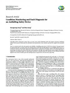
Fig. 1 Architecture of .NET framework
The .NET framework can be regarded theoretically as platform independent at the present time, since Microsoft only provides Windows-based CLR to convert IL into native platform codes despite the fact that IL codes are platform independent. Currently, the third-party Mono project has been designed to allow the .NET developers to easily implement .NET applications on Linux.
.NET FRAMEWORK
The .NET framework is a windows-based software framework provided by Microsoft, which has been regarded widely as a paramount technology in the software world. All other Microsoft technologies in the future are believed to be depended on it. The framework possesses two main components: the common language runtime (CLR) and the .NET framework class library.
III.
FAULT DIAGNOSIS AND FAILURE PROGNOSIS SYSTEM BASED ON .NET FRAMEWORK
The proposed fault diagnosis and failure prognosis system contains four main components: data processing, feature extraction, fault diagnosis and failure prognosis. The four components can be written in any of the .NET languages and executed in real-time in the .NET framework. In this section, we describe the system architecture, and then present a generic particle-filtering-based framework for fault diagnosis and failure prognosis.
Functioning as a software execution environment, the CLR is the foundation of the .NET framework providing a large range of services, such as memory management, thread management, enhanced security, debugging and profiling services, exception handling, code checking and compilation, etc., to aid the system developer during the creation of .NET components. The class library is a comprehensive, objectoriented code collection that can be combined with the developer’s own codes to be used in a variety of applications. Note that this class library can be accessed from any of the .NET languages. Therefore, what all programmers have to learn is only this single library even if different programming languages, such as Visual Basic. NET and Visual C#.NET, etc., are utilized.
A. System Architecture Fig. 2 shows the system architecture. Four system modules with different functionality are built as the respective .NET components. As the foundation of the architecture, the .NET framework provides not only a software runtime environment but also a variety of services that help all of the four components achieve their objective functionality.
Fig. 1 shows the architecture of this framework. The source codes written in any of the .NET languages are compiled into Microsoft Intermediate Language (IL) that is processor independent and can be portable to a number of platforms. A variety of instructions are included in IL for different types of operations, such as loading, storing, initializing, and calling methods on objects, as well as arithmetic and logical
Each .NET component in the system has its own GUI, and can be adopted as an independent subsystem in the application environments. Moreover, one .NET component can be divided into several .NET subcomponents, each one of them designed to implement one specific type of algorithm/model for a class of applications. For instance, the failure prognosis .NET component is divided into multiple subcomponents that relate
37
recursively the current/long-term fault states by taking into account available measurements. Both diagnosis and prognosis contain two key steps: prediction and update. The prediction is intended to estimate the prior probability density function (PDF) of the states by using the following nonlinear system model:
to a variety of engineering systems such as bearing, shaft, gear, etc., as shown in Fig. 3. Each subcomponent employs various fault models to forecast the evolution of fault indicators on the basis of the application type that is chosen by the user via the GUI.
xk = f k ( xk −1 , ωk −1 )
(1)
where xk is the system state vector at time k, ωk −1 is an i.i.d. process noise at time k-1, and f k is a nonlinear function that represents the evolution of the system states with time. Based on the specific type of application, it is noted that a different f k can be chosen for diagnosis and prognosis. The update step involves modifying the prior density to gain the posterior density, through the use of the following measurement model: yk = hk (xk , vk )
(2)
where yk is the measurement vector, vk is an i.i.d. measurement noise, and hk is a nonlinear function that denotes the non-linear mapping between the system states and the noisy measurements. According to the sequential Monte Carlo approach, the posterior density is approximated by
Fig. 2. Architecture of proposed system. GUI is the Graphical User Interface.
(
N
p(xk y1:k ) ≈ ∑ wki δ xk − xki i =1
)
(3)
where N is the total number of particles, wki is the weight of the ith particle at time k, and δ (•) is the Dirac delta measure. The weights are updated as
(
wki = wki −1 p yk xki
)
(4)
In fault diagnosis, the fault state PDF, p(xk y1:k ) , at time k is calculated by using (1)-(4). This PDF is a fault indicator comparing the current state with the baseline state PDF that represents the statistical/historical information about the normal operational states of the system. The statistical confidence of the fault detection can be calculated by the sum of the weights of the particles, whose states xki are larger than z1−α , u ,σ . Here,
Fig. 3. Decomposition of .NET component. GUI is the Graphical User Interface
When the algorithm/model in the component needs to be updated, the new one can be integrated in the original .NET component as an additional class, or developed as a new .NET component without changing the existing one. An alternative method to update the algorithms/models is to adjust the respective parameter values. Note that these values in the .NET components are stored independently as text files and delivered to the user with the corresponding .NET components, which makes the modification process quite easy. All of the abovementioned architecture’s features provide the system with great modularity, flexibility, and easy updating.
z1−α , u ,σ is the threshold value of the baseline state distribution with the mean u , standard deviation σ and a user-specified false alarm rate α .
When a fault is detected, fault diagnosis is stopped and the failure prognosis module is activated. The main purpose of prognosis is to carry out long-term (multi-step) predictions and obtain the remaining useful life (RUL) of the faulty components. The long-term (p-step) predictions can be achieved by successively taking the expectation of the system model (1)
B. Particle-Filtering-Based Fault Diagnosis and Prognosis From a particle filtering perspective [5], real-time fault diagnosis and failure prognosis is aiming to estimate
[ (
)]
xˆk + p = E f k + p xˆki + p−1 , ωk + p −1 , xˆki = ~ xki .
38
(5)
Fig. 4 shows the system for real-time spalling fault diagnosis and failure prognosis. A GUI is developed to access two independent .NET components: fault diagnosis and failure prognosis. The diagnostic and prognostic results are exhibited in real-time in the GUI. The user can set the values of the system parameters in the GUI, such as the number of particles, the forgetting factor and the process model noise, etc. In the GUI, the three subfigures from the left to the right in the Diagnostic Results box show the fault progression, fault PDF and the confidence in failure declaration, respectively. The below three subfigures depict in real-time the fault prediction, PDF of time to failure (TTF) and predicted RUL. On the top right side of the GUI, the System Outputs box presents the indicators of fault diagnosis and failure prognosis, which include type I error, type II error and RUL.
where xˆki + p−1 is the estimated state associated with the ith particle at time k+p-1, ~ x i is the current state of the ith particle. k
The RUL can be computed by N
(
)
RUL = ∑ f t xˆki , H l , H u wki i =1
(6)
where N is the total number of particles, wki is the weight of the ith particle at time k, H l , H u are the lower and upper bounds of the fault size hazard zone, and f t is a function used to calculate the RUL of each particle. IV.
CASE STUDIES
A. Bearing Spalling Fault Diagnosis and Failure Prognosis Spalling is a main fault mode of bearings, which originates as minute cracks, increases in size during operations and finally initiates cracking and/or flaking of the material. In this case, vibration data was sampled at the frequency of 204.8 kHz from a naturally occurring spall. Then features were extracted from an enveloped/modulated segment of the vibration signals in the frequency domain, by taking the sum of the weighted frequency components associated with harmonics of the frequency of interest. Here, the features have been extracted and provided by the customer, who only needs the diagnosis and prognosis .NET components. In many applications, we have noticed that the customer is just expected to acquire some components of the system. Since the developed system consists of independent .NET components, each one with its own functionality and GUI can be delivered to the customer based on the specific requirements. Fig. 4 System for spalling fault diagnosis and failure prognosis
Based on Paris’ Law, the fault propagation model can be expressed by L(t + 1) = L(t ) + θ1 (t )(L(t ))
θ 2 (t )
+ ω (t )
In the program, the fault diagnosis component is activated first. Then, the failure prognosis component is activated once the fault confidence reaches a specified threshold value, for instance, 95%. When a new measurement becomes available, the prognostic component makes long-term predictions for all particles in the particle filtering scheme. When the state of each particle reaches the predefined hazard zone, the respective time instants of the particles can form a real-time distribution of TTF. Based on the PDF of TTF, the RUL can be calculated by subtracting the current time instant from the sum of the product of the weight and predicted TTF of each particle.
(7)
where L is the spalled surface area, and θ1 , θ 2 are the parameters that will be optimized on-line by the recursive least square method [6]. According to (7), the fault diagnosis and failure prognosis can be depicted as the following equations: ⎞ ⎛ ⎡ xd 1 (t )⎤ ⎡ xd 1 (t + 1)⎤ ⎢ x (t + 1)⎥ = f b ⎜⎜ ⎢ x (t )⎥ + n(t )⎟⎟ ⎣ d2 ⎦ ⎠ ⎝⎣ d2 ⎦
(8)
L(t + 1) = L(t ) + θ1 (t )(L(t )) 2 xd 2 (t ) + ω (t )
(9)
⎧⎪ [1 0]T , if x − [1 0]T ≤ x − [0 1]T f b (x ) = ⎨ ⎪⎩[0 1]T , else
(10)
In order to evaluate the performance of the proposed system, the fault diagnosis and failure prognosis modules was executed in another popular software environment--MATLAB, a powerful numerical computing language that has been used widely in industry and the academic world. The system performance comparison is made between the .NET and MATLAB environments.
where xd 1 and xd 2 are Boolean states that represent normal and faulty conditions, respectively, n(t ) is an i.i.d. uniform white noise, and ω (t ) is an i.i.d. process noise.
Table I gives the comparison results. Here, the performance index is divided into four levels: bad, normal, good and excellent. Both .NET and MATLAB have excellent modularity: every system module can be built as an individual component and utilized independently, since they adopt an
θ (t )
39
1) Data Processing: Three-phase currents (Ia, Ib and Ic) and three terminal-to-terminal voltages (Uab, Ubc, Uca) are measured by sensors at a rate of 100 kHz. The current and voltage signals are analyzed in two distinct frequency bands. The first frequency band of interest occurs around the natural lag frequency of the resolver, f1* = 3.05 kHz. The second band
object-oriented programming environment. They also possess good interoperability that enables them to access the codes executed outside the software environments. Since the system programs can be written in any of the .NET languages, .NET shows better flexibility than MATLAB. It is found that the code execution speed of .NET is much faster than that of MATLAB (24 times faster in this case), which suggests that .NET owns better computational efficiency and thus is more appropriate to be implemented on-line and in real-time on practical systems. In most actual implementations, MATLAB code is always converted into C/C++, thus additional tasks, such as recoding, recompilation, redebugging and new GUI development, etc., have to be completed by the user; the .NET components and GUI, however, can be directly deployed and executed on the target computers by using simple XCOPY operations. Since the .NET framework provides a comprehensive and powerful graphical application programming interface (API) called as Windows Forms, the GUI generation becomes an easy and convenient task. TABLE I.
occurs around f 2* , which is related to the speed of the motor fRPM, P f RPM f 2* = (11) 2 60 where P=8 is the number of magnetic poles in the Brushless DC motor. Data acquired from all terminal-to-terminal voltage (Uab, Ubc, Uca) and current signals (Ia, Ib and Ic) are filtered at two ∗ ∗ frequency bands that are related to f1 and f 2 via two IIR butterworth band-pass filters. 2) Feature Extraction: Four features are extracted from the filtered terminal-to-terminal voltage and current data. The first two features are computed as
SYSTEM PERFORMANCE COMPARISON IN .NET AND MATLAB ENVIRONMENTS
Performance Index
.NET
MATLAB
Modularity
excellent
excellent
Flexibility
excellent
good
Interoperability
good
good
Usage Simplicity
excellent
normal
Deployment
good
good
Execution Speed
good
normal
GUI
excellent
good
(
)
(12)
(
)
(13)
3 1 n) f1 = ∑ RMS U1(abc n =1 3 3 1 n) f 2 = ∑ RMS I1(abc n =1 3
where U1 and I1 are related to the preprocessed data using the first band-pass filter, RMS means the root mean square operation. The other two features are given by
B. Brushless DC Motor Turn-to-turn Winding FaultDiagnosis Turn-to-turn winding fault is when the short occurs across one winding. It has been considered as a primary winding fault mode of the motors, since turn-to-turn insulation is always applied with a thin film of polymide so that it degrades easily due to the severe operational conditions. In this case, turn-toturn winding fault is seeded by placing a resistor in parallel to one of the three windings as shown in Fig. 5. In this way, the extent of the winding short can be controlled precisely by changing the resistance. Firstly, real-time measurements are preprocessed on-line. Then the features are extracted to monitor the behavior of the system. By using an appropriate fault process model, the particle-filtering-based diagnostic algorithm is implemented to detect the fault states with a given false alarm rate (Type I Error) and confidence level (Type II Error).
(
3 1 n) f 3 = ∑ RMS U 2(abc 3 n =1
(
3 1 n) f 4 = ∑ RMS I 2(abc n =1 3
)
(14)
)
(15)
where U2 and I2 are related to the preprocessed data using the second band-pass filter. The next step is to map the computed features to the known fault values inserted during the seeded fault test. The features are used with knowledge of the known fault state L to train a three-layer (4-20-1) feed-forward neural network, by using the Levenberg-Marquardt algorithm. Here, when a fault is seeded, L = 1, otherwise, L = -1. After training, the low mean-squared error (MSE), approximately 10-2, is obtained. 3) Fault diagnosis: Since the neural network can not achieve 100 percent fault detection accuracy, and the noise at the neural network output is significant enough to false trigger. To avoid such an event, particle filtering is used as a means to filter the fault estimate L to ensure a user specified false alarm rate and confidence level when declaring a fault. The fault growth model is motivated from the steepest descent (or gradient descent) algorithm used in adaptive filtering, as shown below
Fig. 5 Turn-to-turn winding fault insertion
L(t + 1) = sat (L(t ) + λ (L(t ) − L(t − 1)) + ω (t ), − 1, + 1) (16)
40
where ω (t ) is an i.i.d. process noise, and sat is a saturation operator within the range [− 1,1] . When a change of fault state occurs during two consecutive sampling times, it encourages the state to evolve. Meanwhile, the contribution of the change is restricted by a factor of λ .
Similarly to the bearing spalling case, the system was also executed in the MATLAB environment and compared with the .NET framework. The same performance comparison results, as shown in Table 1, are obtained. It can be seen that the .NET framework possesses better performance in flexibility, usage simplicity, execution speed and GUI. Note that the fault diagnosis .NET component employed in the bearing spalling case can be “borrowed” to be adopted in the current application, except that the fault model needs to be modified while other algorithm routines remain the same. Meanwhile, the .NET subcomponents in this case, such as data processing1, data processing2, feature processing, and feature fusion, can be employed conveniently in other applications after modifying the parameter values in the text files. It suggests that the developed .NET components can be employed not only in the similar applications but also in the various ones with little modification, which apparently exhibits the advantages of modularity and flexibility of the proposed architecture
4) Experimental results: Fig. 6 shows the proposed diagnostic system that includes a GUI and three independent .NET components. The data processing component consists of two subcomponents that perform bandpass filtering related to f1∗ and f 2∗ , respectively. Four features are obtained by using the feature processing subcomponent. They are then fused into one feature through the feature fusion subcomponent via the neural network. The diagnosis component finally gives the filtered fault state with a user specified false alarm rate and confidence level. Note that data processing and feature extraction modules in this case are divided into several .NET subcomponents. It results in a flexible system structure, since each subcomponent can be updated easily in the current application and employed conveniently in other ones, considering that only one algorithm is adopted in each subcomponent and its parameter values are stored independently in the from of TXT.
CONCLUSIONS V. This paper proposes an integrated fault diagnosis and failure prognosis scheme for critical engineering systems. The architecture of the system is based on the .NET framework that provides a variety of features to meet specified performance requirements from both the developer’s and the user’s standpoints. The system involves four .NET components: data processing, feature extraction, fault diagnosis and failure prognosis. Each component can be developed in any of the .NET languages and employed independently. A generic particle-filtering-based framework is integrated in the system to accomplish the fault diagnosis and failure prognosis tasks. The system is evaluated by two different engineering applications, and a performance comparison is carried out with the MATLAB environment. The results demonstrate the effectiveness and efficiency of the system, and better performance, especially from the point of view of the user, can be achieved compared to the MATLAB environment. Therefore, the proposed system is suggested to be employed, as a general fault diagnosis and failure prognosis architecture, for a variety of engineering systems.
Fig. 6 System for turn-to-turn winding fault diagnosis
REFERENCES
On the left side of the GUI, four features are plotted in realtime. The three subfigures from the top to the bottom on the right side of the GUI show the fault progression (the blue and red lines give the estimated fault states before and after diagnosis component), fault residual PDF and confidence of failure, respectively. Type I error and type II error are shown on the top right side.
[1]
[2]
[3] [4]
The results shown in Fig. 6 are generated by a test example that a fault with a 10 Ω resistor was inserted at time 1.5 seconds. The system detects the fault at the time of 1.6 seconds, which is indicated by the subfigure of confidence of failure on the right bottom side of the GUI. As can be seen, the confidence of failure from 1.6 seconds becomes larger than the user specified confidence level (95%). The 0.1 seconds fault detection latency is caused by the fault detection rate. Here, the system updates the fault detection results at the rate of 0.2 seconds.
[5]
[6]
41
G. Vachtsevanos, F. Lewis, M. Roemer, A. Hess, and B. Wu, Intelligent Fault Diagnosis and Prognosis for Engineering Systems. USA: Wiley, 2006. A.K.S. Jardine, D. Lin, D. Banjevic, “A review on machinery diagnostics and prognostics implementing condition-based maintenance,” Mech. Syst. Signal Process., vol. 20, pp. 1483-1510, 2006 D. Chappell, Understanding .NET. USA: Addison-Wesley, 2002. M. Orchard, G. Vachtsevanos, “A particle filtering approach for on-Line fault diagnosis and failure prognosis,” Trans. I. Meas. Control, vol. 31, no. 3-4, pp. 221-246, June 2009. M.S. Arulampalam, S. Maskell, N. Gordon, T. Clapp, “A tutorial on particle filters for online nonlinear/non-Gaussian Bayesian tracking,” IEEE Trans. Signal Process., vol. 50, pp.174–188, 2002. K. M. Passino, Biomimicry for Optimization, Control, and Automation. USA: Springer, 2005.