A Network Abstraction for Control Systems

Technical Report 2014/01

A Network Abstraction for Control Systems Ben W. Carabelli Frank Dürr Boris Koldehofe Kurt Rothermel

Institute of Parallel and Distributed Systems University of Stuttgart Universitätsstr. 38 705679 Stuttgart Germany April 2014

A Network Abstraction for Control Systems Ben W. Carabelli, Frank Dürr, Boris Koldehofe, and Kurt Rothermel Institute of Parallel and Distributed Systems University of Stuttgart, Germany

Abstract Networked control systems (NCS), such as the smart power grid, implement feedback control loops by connecting distributed sensors and actuators to a remote controller over a communication network. In order to avoid the costly and timeconsuming installation of dedicated networks, NCS can benefit from utilizing readily available IP networks such as the Internet. However, as control systems are typically sensitive to delay and loss, the integration of such systems over best-effort networks becomes a challenge, which we address in this paper with two main contributions. First, we propose an end-to-end transport abstraction for NCS based on a novel probabilistic quality of service specification which (1) is compatible with existing control models and (2) provides the network with application-specific knowledge about the relation between system performance and network-relevant metrics. Second, we realize this abstraction at the network layer with an optimal routing algorithm, which fulfils the required QoS while minimizing the usage of network resources. We show that our approach lends itself to the implementation with state-of-the-art software-defined networking (SDN) technologies, and demonstrate its effectiveness in our evaluation. Index terms — cyber-physical systems; networked control systems; optimization; routing; software-defined networking

1

Introduction

Networked control systems (NCS) [HNX07], implementing a feedback control loop by connecting distributed sensors, actuators, and controllers via a communication network, are steadily gaining importance. One prominent example of a widely dispersed NCS is the smart grid, where smart meters or synchrophasor units measure the power consumption of electrical appliances and the production by decentralized sources (e.g., solar panels). The controller balances power generation and consumption by switching on and off consumers on demand. Further examples include autonomous traffic systems, smart factories, smart homes, and several types of so-called cyber-physical systems. Many of those NCS involve widely distributed sensors and actuators, which are to be connected to controllers via a communication network. The areas to be covered by those networks range from single campuses or production sites to the entire globe. A crucial factor for the proliferation of such NCS will be to what extent existing packet-switched network infrastructures can be leveraged by control applications.

1

Building NCS on top of packet-switched networks is a challenging task as those systems are particularly vulnerable to unpredictable delays and packet loss. With regard to their requirements concerning the underlying communication network, we can distinguish between deterministic control models and probabilistic control models. While the former require upper bounds on delay and loss, the latter can account for a certain degree of stochastic delay and loss variability. Due to their stringent delay and loss requirements, deterministic control models are typically implemented using fieldbus networks with deterministic real-time guarantees at the data link layer, such as the well-known CAN and PROFIBUS and more recently Ethernet-based variants such as EtherCAT and PROFINET [GH13]. However, implementing deterministic control models based on a best-effort service as provided by the current Internet is unfeasible. While communication services with guaranteed delay bounds, such as IntServ, would be an appropriate base for building deterministic NCS, we cannot expect them to be widely available. As a consequence, we focus our work on probabilistic control models, which can in principle be applied also when the underlying network is expected to provide besteffort service only. The probabilistic control methods proposed in the literature (e.g., [BA11; BA12; Hee+10; QSG07; Sch+07]) incorporate mathematical network models to enable the rigorous analysis of the NCS performance depending on network parameters. However, although these works present a solid theoretic basis for NCS, they typically do not address the problem of mapping these models to communication services that can be (efficiently) realized in current network infrastructures. Consequently, the integration of packet-switched networks and control system to implement NCS requires cross-cutting research at the intersection of networking and control theory [SA11; KK12]. To this end, we aim at a communication service enabling engineers to design and implement an NCS within their established theoretic framework, but which can also be implemented efficiently on top of IP-based networks. In this paper, we propose a novel communication service tailored to the specific needs of probabilistic NCS. This transport-layer service, called NC-service, enables the sensing devices of an NCS to connect to the NCS controller for transmitting their measurements. When requesting a connection, the control application specifies an NCS-specific Quality of Service (QoS), which is based on a control theoretic performance metric. According to the underlying probabilistic control model [BA12], this performance metric is defined as a function of the acceptable delay (given by the sampling period) and the in-time arrival probability given this sampling period. Since different combinations of sampling period and arrival probability values may result in equal performance, there might exist a number of alternative network paths that (currently) fulfill the performance requirement. This allows the NC-service to select the path that allows the maximal sampling period, which in turn minimizes the volume of samples to be transferred. Moreover, the path may be dynamically changed to avoid violating the required performance, or if an alternative path allows for a larger sampling period. Consequently, for a given performance requirement the NC-service determines the optimal sampling period based on the current network conditions. This value is reported to the NCS, which then adapts its sampling process accordingly. Selecting the optimal path based on the performance metric mentioned above requires a customized routing mechanism. However, we can utilize state of the art software-defined networking (SDN) technologies to implement this mechanism, making it applicable to standard networking infrastructures. Moreover, we think that the presented NC-service is well suited to demonstrate the core benefits of SDN, namely, the flexibility to add new network control logic, ease of implementing a logically 2

Control System

NCS-Controller

actuators

Plant sensors

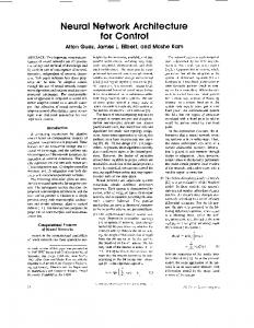
Figure 1: System model; the sensors are connected to the NCS-controller over a network. centralized network service, and integration of the application and network into a holistic system. To our knowledge, this is the first proposal of a communication service incorporating a control-theoretic performance metric, which is in line with the application’s control model, and which allows the service to satisfy the required performance with minimal network resources. In detail, we make the following contributions: • An end-to-end transport abstraction for connecting components of an NCS. • The formal specification of a constrained optimal routing problem to optimally utilize network bandwidth resources subject to QoS constraints. • An SDN-based architecture and logically centralized implementation of the network control logic. • An evaluation of the performance of our approach that shows the feasibility of implementing a logically centralized routing algorithm for a large number of concurrent connections. The remaining paper is organized as follows. We first introduce our system model in Sec. 2 and propose an SDN-based architecture for the NC-service in Sec. 3. After deriving the QoS requirements of a canonical control system, we describe the transport layer functionality in Sec. 4. We then show an efficient implementation of this service on the network layer by formulating and solving an optimal routing problem in Sec. 5. After evaluating our approach with a simulation study in Sec. 6, we address related work in Sec. 7. A discussion of our results and an outlook conclude this work. Further technical details and proofs can be found in the Appendix.

2

System Model

Our system model, which is shown in Fig. 1, consists of five components: the plant, sensor, actuator, NCS-controller, and communication network. According to the common terminology used in control theory, the dynamic physical system to be controlled is denoted as the plant. The current state of the plant is measured by sensors, and corrective actions to the plant are performed through actuators. The NCS-controller receives the input from the sensors, calculates the corrective action required to keep the plant in the desired state, which it sends to the actuators to be executed. In this work, we consider systems with one sensor node only, where the measurements of all sensors are aggregated into a state vector and sent to the controller. Since the plant is a spatially distributed system in general, we assume that the sensor node is connected to the NCS-controller over a communication network. We assume an IP-based packet-switched network with best-effort forwarding semantics. 3

Application Layer Transport Layer

NCS Controller NC Transport Entity

NCS Sensor route setup route delete

NC Socket signaling

NC Routing Service

Network Layer

IP Entity

SDN Network Controller

Data Link & Phy. Layer

link monitoring OpenFlow conn. req.

Data Path

Northbound Interface Southbound Interface

NC Transport Entity IP Entity

conn. ack. data

Figure 2: Network Architecture; NC-service components are shown with bold borders. Therefore, state measurement vectors can get lost with variable loss probability and experience a variable delay. For the sake of simplicity, we assume that the actuators are co-located with the NCS-controller. More complex settings where also the actuators are connected to the NCS-controller over the network are subject of future work. Therefore, our focus in this paper is on the connection between the sensor node and the NCS-controller. For the packet-switched network, we assume the availability of standard multi-layer switches that can forward flows based on IP addresses and higher layer information. Moreover, they have to support the OpenFlow standard [McK+08] for configuring forwarding tables and enabling our SDN-based architecture described next.

3

Network Architecture

The network architecture of our NC-service is depicted in Fig. 2, which shows the relevant components in the five-layer Internet model. As previously mentioned, our proposed NC-service provides a transport layer interface to the control application and utilizes a custom routing mechanism to implement the route of the corresponding NC-connection at the network layer. The transport functionality of the NC-service is implemented by protocol entities on the end-systems hosting the sensor and NCS-controller. We denote the interface between the application and the NC-service as an NC-socket similar to classic sockets for datagram and streaming services. The transport layer service is responsible for setting up an NC-connection between sensor and NCS-controller, tearing down connections, data transfer, QoS arbitration, and signaling changes in network conditions to the application as detailed in the following sections. In order to set up an NC-connection with a given QoS, a network path with certain loss and delay properties has to be established in the network, which might be adapted during the life-time of the connection due to changing network conditions. The setup and maintenance of routes implementing the required QoS with minimum network resources is the task of the NC routing service. According to the SDN paradigm, we implement this service using a logically centralized SDN network controller, which exposes the routing service to the transport layer through its northbound interface. To calculate a route, the NC routing service obtains necessary QoS information from the transport layer entity and gathers a global view onto the network through monitoring of the link properties over the southbound SDN interface, e.g., using counters to detect lost packets or active probing to determine delays. Based on this global view, the NC

4

routing service implements the optimal route in the network by installing the necessary flow table entries in the OpenFlow-enabled switches (based on the IP addresses and port numbers of NCS-controller process and sensor process and protocol ID of the NC transport protocol). Whenever the routing service adapts the route or identifies the need to adjust application parameters in order to maintain QoS, these changes are signaled back to the transport layer. Note that route adaptations can be performed in a non-disruptive fashion using techniques for consistent network updates, e.g., [Rei+12]. Data packets follow the usual data path through the protocol stack. Note that the proposed network architecture does not require changes to the network switches as long as they implement the OpenFlow standard (and possibly other standard mechanisms such as hardware timers for precise delay monitoring). To deploy the service, we only have to modify the protocol stack of the hosts—which are under the control of the NCS-operator—, and deploy custom network control logic via the SDN controller. Therefore, we can use a standard SDN infrastructure.

4

NC Transport Service

We now proceed to design a suitable transport abstraction for NCS, which will be provided by the NC-service. In particular, this abstraction includes the QoS definition used to set up NC-connections. On the one hand, the QoS definition has to provide the network with suitable information to efficiently implement NC-connections on the network layer, i.e., to solve the routing problem. To this end, it must be specified in network-relevant metrics. On the other hand, the QoS parameters must be in line with the control model of the NCS application itself. In order to define a suitable QoS specification for NCS, it is therefore essential to first understand the requirements and relevant parameters of the control application.

4.1 Control-theoretic Background In order to design an NCS, the control systems engineer uses a mathematical model of the plant and the communication network that transmits sensor values from the sensor to the NCS-controller. In this work, we adapt an NCS model of Blind and Allgöwer [BA12], which is described within this subsection. For the communication between sensor and NCS-controller, this model assumes a constant delay TS and arrival probability pa . Furthermore, losses are assumed to be independent and identically distributed (i.i.d.). The plant is modeled using an ordinary differential equation x˙ (t ) = Ax (t ) + Bu (t ) + w (t ),

(1)

where x is the state vector of the plant, which is measured by the sensor, u is the input vector of the plant, and w is a random disturbance which may capture uncertainties, noise, or unmodeled dynamics. As the measurement signal u (t ) has to be packetized in order to be transported over the network, the sensor is sampled periodically at time instants tk , where tk +1 = tk +TS . That is, the network delay TS of the network model is simultaneously the system’s sampling period. According to the model, at each of these sampling instants, two actions are performed: 1. The sensor takes a measurement of the state x and sends it to the controller over the network. The measurement is delivered at the next sampling time tk +1 with probability pa . 5

2. If the controller receives the previous measurement x (tk −1 ), it uses this value to calculate a prediction xˆ (tk ) of the current state. If the last measurement is not available at this time, it uses its previous state estimate xˆ (tk −1 ) instead to calculate the current state estimate. This value is then used to obtain the control input u (t ) = −K xˆ (tk ), t ∈ (tk ,tk +1 ], which is applied by the actuator over the following sampling period. For the details of the state prediction and calculation of the controller gain matrix K see [BA12]. However, it is important to note that this controller is designed to solve the so-called linear-quadratic regulation (LQR) problem, which is among the most prevalent problems in optimal control theory (cf. [Son98]). The LQR controller minimizes a cost metric of the control system, denoted in the literature as J , which measures the deviation of the plant’s state from its setpoint plus the amount of energy that the controller has to expend to stabilize the system. (For technical details see Appendix A.1.) As the system is subject to random disturbances and random packet loss, the cost J is also a random variable. However, the expected value of J under optimal control can be determined numerically as shown in [BA12] as a function of the sampling period  and  the arrival probability. In the following, we denote this function as E[J ] = E J TS ,pa . (Higher moments of J are usually not considered.)

4.2 QoS Specification We can now use the previously described models to relate the application performance to the network parameters. From an application perspective, the control engineer wishes the NCS to maintain a certain performance. She therefore provides an upper bound Jmax for the application’s expected cost:   E J TS ,pa ≤ Jmax . (2) Given this constraint, we can specify QoS for NCS as the required minimum arrival probability given TS : Definition 1. (Minimum Arrival Probability for NCS) The minimum arrival probability function of an NCS with upper cost bound Jmax is given by       (3) pmin TS = inf pa | E J TS ,pa ≤ Jmax . As we have seen in the previous subsection, the delay TS and arrival probability pa can be seen as input parameters to the NCS model. The function pmin now defines a meaningful relationship between these two parameters from the viewpoint of the application’s performance. In order to implement QoS for NC-connections, we must also consider the interdependency of these two parameters at the transport layer. Recall that, in the control model, the packet delivery time of state measurements from sensor to controller is assumed to be constant. From the application perspective, this model is perfectly justified since sensing and actuation only occur at predefined time instants. In the network we must however account for varying delays. State measurements experiencing a delay of less than one sampling period TS can be buffered at the transport layer until the next sampling instant, but those experiencing a greater delay must be discarded, as 6

by this time the controller has already applied an input u based on a state prediction. Effectively, the application parameter pa describes the probability of timely end-to-end delivery of NCS packets within the delay bound TS .1 We can use this effective arrival probability to characterize an NC-connection: Definition 2. (Effective Arrival Probability) Let σ denote an end-to-end NC-connection from sensor to NCS-controller, which imposes a random delay τ σ and random packet σ . The effective arrival probability p (t ) of this connection is loss with probability ploss σ defined as     σ pσ (t ) = P τ σ ≤ t · 1 − ploss , (4)

with respect to the delay bound t.

Thus, an NC-connection satisfies the quality of service requirements of the NCS if we can find a finite positive sampling time TS such that the effective arrival probability exceeds the required minimum arrival probability: ∃TS >Tmin

pσ (TS ) ≥ pmin (TS ),

(5)

where we also include a lower bound Tmin on the allowable sampling period as a design parameter in order to limit the data rate of the NCS traffic. Note that expressing QoS as a function of the application-layer parameter TS has interesting benefits in our scenario: it allows the network to choose an optimal sampling period based on the current network delay and loss such that the NCS requirements are fulfilled with minimal induced network load as we will present in Sec. 5. By using this lightweight but expressive interface, we retain all the degrees of freedom (TS and network path), while providing separation of concerns between the control application and network, allowing for a clean layered design.

4.3 NC Transport Service Interface As outlined in Sec. 3, NC-sockets are used by the NCS-controller and sensor to communicate via an NC-connection. The API specifies operations for opening and closing NC-connections including the required QoS, sending and receiving sensor data, and signaling events between network and NCS, e.g., when the QoS cannot be fulfilled anymore. In the following, we describe the NC-socket interface based on a slight modification of standard socket primitives as well as the transport service semantics. • s = connect( addrsens , pmin (·), *TS , *t 0 , *h ): the NCS-controller (acting as client process) requests an NC-connection to the sensor (acting as server process), providing the IP address and port number of the sensor process as addrsens and the required QoS function pmin (·) as introduced above. During connection establishment, the sampling period is provided via the pointer *TS , and the reference time *t 0 of the NCS is initialized. Both of these values are used to determine the subsequent sampling times of the control system. Due to the sampling semantics of the control application described earlier, we require physical clock synchronization between the two end-systems to define t 0 , which can be achieved using standard technologies like NTP, PTP, or GPS. Furthermore, the NCS-controller provides a signal handler h, which is called by the NC-service whenever the sampling time TS has to be adapted in order to maintain QoS, in 1 Notice the dual semantics of the parameter T : as a sampling period and as a delay bound. This will be S of interest for the optimal routing problem, as it implies an inter-dependency between delay and data rate.

7

which case the reference time t 0 is also reinitialized. The primitive returns the socket descriptor s or -1 if no feasible route could be found. • s = accept( *TS , *t 0 , *h ): the sensor process accepts connections initiated by the NCS-controller. Again, after the connection has been established, the same sampling period TS and reference time t 0 is provided to the sensor process as well as to the NCS-controller, and the sensor provides a handler h to receive signals about sampling period adaptations from the NC-service. The sensor will start sending measurements to the NCS-controller at sampling times tk = t 0 + k · TS . • status = send( s, x ) is the primitive for sending the state vector x measured by the sensor to the NCS-controller. The transport entity encloses a sample number k = ⌊TS−1 (t − t 0 )⌋ corresponding to the current sampling time tk when the measurement was taken. The status signals success or an error, e.g., a broken connection. Note that a connection only breaks if no alternative route for the NC-connection can be found anymore fulfilling the requested QoS. As long as an alternative route can be found, adaptations are signaled via the signal handler h. • status = receive( s, *x ) is the primitive used by the NCS-controller to receive a sample from the sensor. This call blocks until the system receives a packet with valid sample number k = ⌊TS−1 (t − t 0 )⌋ of the most recent sampling time. Older packets must be silently discarded. If no valid packet is received by the next sampling time tk+1 = t 0 + (k + 1) · TS , a timeout error is signaled and the NCS-controller performs a state prediction as shown in Sec. 4.1. This call also returns an error if the NC-connection breaks. • close( s ) closes an NC-connection. Due to the time-bound semantics of the send() and receive() primitives, the transport service does not have to provide sequencing, as only one valid packet can be in transit within any given sampling period, and invalid packets are discarded. Furthermore, delivery acknowledgment and packet retransmission functionality are also unnecessary. For the sake of completeness, we also briefly describe the northbound interface of the NC routing service executed by the Network Controller. These primitives are used by the transport service to pass NC-connection requests down to the network layer, as shown in Fig. 2: • setup_route( addrncsctl , addrsens , pmin (·), *TS ) is used to set up a route from the sensor to the NCS-controller. This interface provides the means to pass the QoS function pmin (·) to the routing service, and correspondingly return the sampling period TS determined by the routing algorithm. • delete_route( addrncsctl , addrsens ) removes flow table entries of a previously established NC-connection. In the following section, we describe in detail how routes are calculated by the NC routing service.

5

NC Routing Service

Based on the QoS definition of NC-connections, we can now focus on the problem of finding optimal network paths for forwarding packets of an NC-connection (or for short NC-flows) such that the requested QoS is fulfilled and the network load is minimized. To this end, we define a formal routing problem for NC-flows in this 8

α νs

τ

ν1

  P α =1   = P ν 1, ν 3

ν2 ν4

ν3 1

νc

    P τ ≤ t = L (ν 1, ν 3 ), t

ν5

0

τ¯ (ν 1, ν 3 )

t

Figure 3: Network model for NC-flow implementation. Each link e ∈ E obeys a distinct random packet loss process α with arrival probability P (e), and a distinct random delay process τ with latency distribution L(e, ·). section after first introducing the prerequisites for this formulation, namely, a formal network model and definitions of the latency and loss properties of network paths as well as network load. Finally, we present an optimal routing algorithm for NC-flows.

5.1 Network Model   We model the communication network as a directed graph G = V ,E, P, L as depicted in Fig. 3. It comprises a set V of vertices modeling network nodes (multi-layer switches or hosts), and a set E ⊆ V ×V of directed edges modeling network links between nodes. G contains two special nodes: νs representing the sensor node, and νc representing the host of the NCS-controller; all other nodes are switches. The map P : E → [0, 1] describes the arrival probability of each link e ∈ E, and L : E × R+ → R+ represents the cumulative distribution function (CDF) of each link’s latency. As notational shorthand for the corresponding probability density functions (PDF), we write ℓ(e,t ), i.e., t L(e,t ) = 0 ℓ(e,τ ) dτ . The transmission of NCS packets is modeled by a stochastic process {α ke ,τke }k ∈N for each link e ∈ E. Here, α ke ∈ {0, 1} is a random binary variable representing packet arrival, i.e., α ke = 0 iff the measurement x (tk ) is dropped on link e, and τke ∈ R+ denotes the random network delay of x (tk ) on link e, assuming it was not lost. As stated above, the stochastic properties of this process are defined by G:   P α ke = 1 = P (e), (arrival prob.) (6)   e + P τk ≤ t = L(e,t ), t ∈ R . (latency dist.) (7)

In accordance with the control model, we assume that the process {α ke ,τke } is independent and identically distributed (i.i.d.) between sampling instants tk and independent over all links.2 Further, let the mean latency of link e ∈ E be denoted by τ¯ (e) = E[τke ]. In order to obtain the properties of NC-flow routes as link sequences, we define   a k-hop path as a tuple of the visited nodes σ = ν 1 ,ν 2 , . . . ,ν k +1 ∈ V k +1 . For k ≥ 1, 2 Note that loss and delay are also assumed to be mutually independent. However, the delay of lost packets is neither observable  nor does it have  any influence on the control application, which renders the conditional probability P τke ≤ t | α ke = 0 irrelevant. Therefore, this assumption is clearly justified.

9

  a path must be connected in G and thus satisfy ν i ,ν i+1 ∈ E for all i = 1, . . . ,k. For k = 0 the path reduces toa single node,which we refer to a as a degenerate path. We  m 2 1 1 say that two paths σ1 = ν 1 ,ν 1 , . . . ,ν 1 and σ2 = ν 2 ,ν 22 , . . . ,ν 2n are adjacent if the terminal node of the first coincides with the initial node of the second, i.e., ν 1m = ν 21 . The concatenation of two adjacent paths is denoted as σ1 ◦ σ2 = ν 11 ,ν 12 , . . . ,ν 1m ,ν 22 , . . . ,ν 2n . Finally, we say that two distinct paths are parallel if the initial and terminal nodes of both paths coincide, i.e., ν 11 = ν 21 and ν 1m = ν 2n .

5.2 Path Properties By regarding the stochastic properties of link concatenation with respect to delay and loss, P and L can also be extended to paths. For the sake of consistency, we consider any degenerate path σ ∈ V as a perfectly reliable and instantaneous link, i.e., P (σ ) = 1, L(σ ,t ) ≡ 1, and τ¯ (σ ) = 0. Proposition 1. Given two adjacent paths σ1 and σ2 , the overall arrival probability and delay probability density of the composite path σ1 ◦ σ2 are given by   P σ1 ◦ σ2 = P (σ1 ) · P (σ2 ) (8)   and ℓ σ1 ◦ σ2 ,t = ℓ(σ1 ,t ) ∗ ℓ(σ2 ,t ), (9)

where ∗ denotes convolution with respect to t.

(Proof cf. Appendix A.2.) Note that we can express the effective arrival probability of NCS packets over a path σ in G as pσ (TS ) = P (σ ) · L(σ ,TS ). Obviously, the above proposition implies:   ( ) P σ1 ◦ σ2 ≤ min P (σ1 ), P (σ2 )   ( ) and L σ1 ◦ σ2 ,t ≤ min L(σ1 ,t ), L(σ2 ,t ) , ∀t ∈ R+.

That is, the effective arrival probability of a composite path cannot be larger than those of its constituents.

5.3 Load Metric Next, we introduce the network load metric used in our optimization criterion. Taking into account the stochastic f g nature of our link model, we use as a load measure the expected value L = E b ·τ σ of the bandwidth–delay product, where b is the data rate of the traffic generated by the control application and τ σ is the random latency of the path. We can see, however, that the naïve calculation of this load measure as b · τ¯ (σ ) is overly pessimistic, as it disregards the possibility of packets being dropped. On the other hand, if we simply weigh the naïve measure with the path arrival probability, i.e., b ·τ¯ (σ ) ·P (σ ), the result is overly optimistic, as even in the case of a packet loss, this loss might not occur at the beginning of the path. Thus, a packet lost along the way may still incur a partial network load. In order to accommodate these considerations, we use the following path metric to capture the expected delay experienced by any packet along a given path. Definition 3. (Expected transit time) The expected time that a packet spends in transit on path σ = e 1 ◦ e 2 ◦ e 3 ◦ · · · in G is  ! def Eτ (σ ) = *τ¯ (e 1) + P (e 1) · τ¯ (e 2) + P (e 2) · τ¯ (e 3) + . . . +. , 10

τ¯ = 1 P = 0.1

ν2

τ¯ = 1 P = 0.9

ν1

σ ν4

τ¯ = 1 P = 0.9

ν3

τ¯ = 1 P = 0.1

  ν ,ν ,ν  1 2 4 ν 1, ν 3, ν 4

  τ¯ σ

  P σ

  Eτ σ

2

0.09

1.1

2

0.09

1.9

Figure 4: Expected transit time This metric is also demonstrated in Fig. 4, which shows a minimal example of two parallel 2-hop paths with identical end-to-end characteristics. We see that the path via ν 2 with the less reliable link on the first hop incurs a shorter expected transit time and thus lower expected network load. Similar metrics have previously been investigated in the context of energy-efficient routing in wireless sensor networks, cf. [Sau+06]. Note that the expected transit time of any link e ∈ E is simply its mean delay Eτ (e) = τ¯ (e) and that of a degenerate path σ ∈ V is Eτ (σ ) = 0. Also, given two adjacent paths σ1 and σ2 , the expected transit time of the composite path σ1 ◦ σ2 is   Eτ σ1 ◦ σ2 = Eτ (σ1 ) + P (σ1 ) Eτ (σ2 ), (10)

which follows directly from Definition 3. As the data rate of the traffic generated by the control application is inversely proportional to the sampling period TS , the induced network load on path σ with sampling period TS is given by L(σ ,TS ) = Eτ (σ )/TS .

5.4 Routing Objective Based on the formulation of the network load L(σ ,TS ), we can now define our constrained optimization problem. Recall that NCS-QoS requires that for some TS ≥ Tmin , the minimum arrival probability function pmin (TS ) of the NCS be exceeded by pσ (TS ), which defines the probability of receiving a sample in time considering the loss and delay distribution of the path σ . In order to minimize the network load, we are interested in the maximal feasible sampling period given by ) (   sup t >Tmin pσ (t ) ≥ pmin (t ) if exists  Tmax (σ ) =  otherwise. 0

Informally, the sampling period can be increased (i.e., the sampling rate is decreased) as long as the QoS requirements are still satisfied. If the loss and/or delay of a path is −1 too high, the path is unfeasible, i.e., even choosing the maximum sampling rate Tmin cannot compensate for the insufficient path quality. In this case we define Tmax = 0, corresponding to infinite load. Note that the expected transit time only depends on the choice of path, but not on the sampling period. Therefore, the load on any given path is minimized by choosing TS = Tmax (σ ), and we denote this minimal per-path ˜ ). load as L(σ Now we are ready to formulate an optimization problem for NC-flow routing, where we determine a path from the sensor node νs to the controller node νc with minimal network load: ˜ ) = Eτ (σ ) s. t. σ1 = νs , σn = νc . min L(σ σ ∈G Tmax (σ )

(11)

Note that any path σ for which QoS cannot be satisfied has Tmax (σ ) = 0 and therefore ˜ ), rendering it unfeasible. incurs infinite network load L(σ 11

5.5 Routing Algorithm Being a constrained shortest path problem, the considered routing problem (11) belongs to the class of NP-complete problems (cf. [Zie01]). Moreover, the QoS constraint (5) is not expressed in terms of a scalar constraint metric; therefore, traditional approximation methods for constrained shortest path problems are not readily applicable. However, we employ a dynamic programming approach and show that its application is practicable on a realistic topology in Sec. 6. Our algorithm is shown in Fig. 5. We maintain for each node νi a set R(νi ) of residual candidate paths to the target node νc , which is initialized in lines 2–5 as empty for all nodes except the NCS-controller node, where it contains the degenerate path (νc ). We then successively generate simple paths from each node towards νc by relaxation of each node’s incoming edges in lines 6–14. Upon relaxing an edge (νi ,ν j ) in lines 18–32, we evaluate for each path σ ∈ R(ν j ) the extended path σˆ = νi σ . As the set of simple paths to any node in G scales with O(|V |!) in the worst case, we would want to avoid generating all these paths. Due to the problem structure, we can unfortunately not select the ‘best’ path at every step as would be possible in an unconstrained shortest path problem. We can, however, identify non-optimal subpaths using a necessary optimality condition given in the following proposition. Proposition 2. Consider two parallel paths σ1 and σ2 from any node νi to the controller node νc . If these paths satisfy P (σ1 )L(σ1 ,t ) < P (σ2 )L(σ2 ,t ), ∀t and

Eτ (σ1 ) > Eτ (σ2 )

(12) (13)

then the solution σopt of the optimal routing problem (11) cannot contain σ1 as a subpath. (Proof cf. Appendix A.3.) Based on this result, we can safely discard paths which meet the following condition as route candidates. Definition 4. (Dominance) If two parallel paths σ1 and σ2 satisfy both (12) and (13), then we say that σ2 dominates σ1 . As notational shorthand for this case, we write σ2 ≫ σ1 . Specifically, in lines 21–27, we discard the candidate σˆ if it contains a loop, is unfeasible, or dominated by any existing path in R(νi ). Otherwise, we know that it is eligible as subpath of the optimal solution, and we add it to R(νi ). In line 28, we also purge R(νi ) of all paths which are dominated by the newly added σˆ , in order to further minimize the required number of relaxation steps. After a new candidate path was added to the set R(νi ), we schedule in line 30 the incoming edges of νi to be relaxed in the main loop. Thus, each R(νi ) converges to a set containing all feasible, non-dominated simple paths from νi to νc . Finally, when no edges are left to be relaxed, we can choose in line 15 from all candidate paths in R(νs ) the one with the minimal cost L, which constitutes the optimal solution. If the removal of dominated paths should not prove sufficient to limit the practical complexity of the algorithm, we would first try to obtain a control-feasible path which does not necessarily minimize network load. This can be achieved for example by employing a suboptimal variant of the routing algorithm, which replaces the expected transit time Eτ (σ ) by the unweighted mean path delay τ¯ (σ ), and relaxes the strict inequality in (13). This approach leads to a larger number of discardable dominated paths, as we show briefly in the evaluation. 12

Require: G = (V ,E, P, L) – network graph pmin (·) – minimum arrival probability (provided by application) νs ,νc ∈ V – sensor and controller node Ensure: σopt solves (11) 1: 2: 3: 4: 5: 6: 7: 8: 9: 10: 11: 12: 13: 14: 15: 16: 17: 18: 19: 20: 21: 22: 23: 24: 25: 26: 27: 28: 29: 30: 31: 32:

function OptimalRoute(G, pmin (·), νs , νc ) for all nodes νn ∈ V do R(νn ) ← ∅ end for ⊲ initialize path set on νc R(νc ) ← {νc } M ← {νc } ⊲ mark νc for relaxation repeat for all νn ∈ M do for all νi with (νi ,νn ) ∈ E do Relax(νi ,νn ) end for ⊲ unmark node νn M ← M \ {νn } end for until M = ∅   σopt ← arg min σ ∈R (νs ) Eτ (σ )/Tmax (σ ) return σopt end function function Relax(νi ,ν j ) for all σ ∈ R(ν j ) do ⊲ new candidate path σˆ ← νi σ if νi ∈ σ or σˆ ∈ R(νi ) ⊲ loop/duplicate continue calculate Eτ (σˆ ), P (σˆ ), and L(σˆ ,t ) if P (σˆ )L(σˆ ,t ) < pmin (t ) ∀t >Tmin ⊲ σˆ unfeas. continue ⊲ σˆ dominated if ∃ σ ∈ R(νi ) : σ ≫ σˆ continue ⊲ purge R(νi ) R(νi ) ← R(νi ) \ {σ | σˆ ≫ σ } R(νi ) ← R(νi ) ∪ {σˆ } ⊲ add σˆ to R(νi ) M ← M ∪ {νi } ⊲ mark νi for relaxation end for end function Figure 5: NC-flow Routing Algorithm

6

Evaluation

In this section, we evaluate the performance of our approach using network simulation. In detail, we evaluate the effectiveness of our NC-service for networked control, the efficiency of network optimization using our routing algorithm, and the runtime performance of this routing algorithm. We begin by introducing our evaluation setup, before we present the results.

13

m

m·д

Linearized ODE model: " # " # #" " # 0 1 θ (t ) 0 θ˙ (t ) = + u (t ) 1 0 θ˙ (t ) 1 θ¨(t ) | {z } | {z } | {z } |{z}

θ

A

x˙ (t )

u

x (t )

B

Figure 6: Inverted pendulum system with linear differential equation model. The state comprises angle θ and angular speed θ˙. The plant’s input u is the torque applied to the pendulum.

6.1 Simulation Environment For the first two studies, we simulated the integrated NCS consisting of the network, the control system, and the previously described network control logic under different scenarios. We used the OMNeT++/INET simulation environment [VH08] for the eventbased simulation of the communication network. The controller synthesis and stepwise simulation of the control system were implemented using the GNU Octave scientific computing language [EBH08], which was integrated with the network simulator using Octave’s C++ API and runtime library. 6.1.1

Simulation of the Control System

For our evaluation of the closed-loop system, we simulated a textbook example of an unstable physical system, namely, the inverted pendulum system depicted in Fig. 6. The state of that plant is given by the angle θ of the pendulum with respect to the upright position, and its angular speed θ˙. The pendulum is in equilibrium in the upright position θ = θ˙ = 0, but will tip over if disturbed; it is therefore an unstable system. Our goal is to efficiently apply a torque u at the base of the pendulum depending on the state such that it is kept in an upright position despite disturbances, which are modeled as additive Gaussian white noise. In the context of our investigated NCS setup presented in Fig. 1, one might assume, e.g., that we measure the angle and speed of the pendulum using a remote camera, which sends its state measurement to a controller connected to the actuator at the base of the pendulum. If we use the control scheme from [BA12], we will obtain a controller minimizing the cost function 1 J = lim T →∞ T



T

θ (t ) 2 + θ˙ (t ) 2 + u (t ) 2 dt .

0

The terms under the integral ensure that the angle and speed of the pendulum as well as the torque applied are kept small on average. The control-theoretic framework allows us to predict the expected value of J for this system depending on the parameters pa and TS . For our simulation study, we assume that a performance bound of Jmax = 1 was prescribed by the application. From this we derive the minimum arrival probability function, which for this system is shown in Fig. 7, as explained earlier in Sec. 4. The figure shows that the sampling period should be no longer than approximately 57 ms if the quality requirement is to be satisfied. We also added plots of pmin for other values of Jmax for comparison.

14

1 J J J J

0.8

= 0.9 = 1.0 = 1.1 = 1.2

pmin

0.6

0.4

0.2

0 0

10

20

30

40

50

TS [ms] Figure 7: Numerically obtained minimum arrival probability function pmin (TS ) for the inverted pendulum shown in Fig. 6 at different performance levels of J . Rb

νs

ν1

Rb C link

ν2

Rb C link

ν3

C link

ν4

νc

Figure 8: Linear topology used to study the validity of our network abstraction. 6.1.2

Simulation of the Network

In order to simulate our NCS, we implemented two applications for OMNeT++: a PlantApp containing the sensor, and a ControllerApp implementing the NCScontroller. Both applications are executed on different hosts in the IP network. After each simulation step of one sampling period, the PlantApp sends a packet containing the state vector x and sample number k over the network to the ControllerApp. This vector is used to calculate the control input in the next simulation step or discarded based on its sample number. The network configuration is performed by a separate module (Config) which maintains a topology model, as well as loss probabilities and latency distributions in the form of discrete empirical CDFs with 100 bins each. These distributions are calculated based on queue time statistics from the network interfaces of switches, which the Config module receives through the signal mechanism of OMNeT++. Each experiment is preceded by a 5 s monitoring period during which the Config module measures delay and loss. It then executes the optimal routing algorithm, installs the appropriate routing table entries for the NC-flow, and sends an initialization message containing the sampling time TS to the PlantApp, which then begins the control system simulation.

6.2 Effectiveness of NC Service In order to evaluate the effectiveness of our NC-service for network control systems communicating over best-effort IP networks, we simulated the inverted pendulum NCS introduced above with a 5-hop linear topology shown in Fig. 8. Nodes νs and νc 15

1.6 1.4

J L

1.2 1 0.8 0.6 0.4 0.2 0 0.2

0.3

0.4

0.5 Rb /C link

0.6

0.7

0.8

Figure 9: Sample mean of measured control cost J and load L of the NCS traffic depending on the data rate of regular cross-traffic sources with 95% confidence interval. host the PlantApp and ControllerApp, respectively, and nodes ν 1 –ν 4 are intermediate switches. At each switch ν 1 –ν 3 , we inject random UDP traffic with uniformly distributed inter-arrival times and mean bit rate Rb to introduce varying queueing delays and packet losses due to tail drop queueing. As the routing algorithm cannot switch to a lightly loaded path in this topology, we can observe the effective application performance under different levels of network congestion. To this end, we simulated the NCS for different values of Rb , and measured the average control performance J and load L induced by the feedback traffic of the control application. Figure 9 shows these quantities in dependence on the cross-traffic bit rate as a fraction of the link capacity C link . As we can see, the use of the sampling rate determined by our NCS-QoS model is effective at satisfying the targeted quality constraint Jmax = 1 for a large range of cross-traffic levels up to Rb ≈ 0.5 · C link . Moreover, performance degrades gracefully under increasing congestion beyond this value. (Note that already a cross-traffic bitrate of Rb ≥ 0.5 · C link leads to full utilization of the links from ν 2 to ν 4 .) We can also observe how the load L of the application traffic rises gradually due to the adaptation of the sampling period. As the inference of end-to-end latencies is based on the assumption that the link latencies are i.i.d., we also investigated the effects of this assumption being violated, i.e., with strongly correlated traffic. We repeated the above experiment with a mix of regular and bursty (on-off) cross-traffic in equal parts, with traffic bursts lasting 1 s on average. Figure 10 shows that, also for bursty traffic, we could reach the targeted NCS performance for cross-traffic levels up to Rb ≈ 0.5 · C link . Beyond this value, the performance degradation of the NCS due to congestion becomes more pronounced. This is to be expected given the higher sensitivity to varying losses for lower sampling periods (as can be seen from Fig. 7).

6.3 Effectiveness of NC Routing Service In order to investigate the effectiveness of NC-flow routing, we simulated the same NCS with the topology shown in Fig. 11, which offers two possible routes from νs 16

1.6 1.4

J L

1.2 1 0.8 0.6 0.4 0.2 0 0.2

0.3

0.4

0.5 Rb /C link

0.6

0.7

0.8

Figure 10: Sample mean of measured control cost J and load L of the NCS traffic depending on the data rate of bursty cross-traffic sources with 95% confidence interval. ν4 νs

ν1

ν5 ν2

ν3

νc

Figure 11: Network topology used to study the effectiveness of NCS-QoS-routing. to νc . From the beginning of each experiment, we injected at each switch random UDP traffic with uniformly distributed inter-arrival times inducing approximately 80% link utilization on all links, except for the link from ν 1 to ν 4 , which is fully utilized on average. As a consequence, the NC-flow is initially routed over the shorter and less heavily loaded path (νs ,ν 1 ,ν 2 ,ν 3 ,νc ). At t = 20 s after the initial connection setup, an additional traffic source was added from ν 2 to ν 3 , effectively doubling the utilization of this link. As a consequence, the arrival probability of this link decreases and the NCS-QoS requirement is violated, which is detected by estimating the effective arrival probability of the established NC-connection at the transport layer using an exponential moving average of the inter-loss times (where a loss is equivalent to a receive()-timeout). When pσ (TS ) degrades by more than 10%, the NC-service adapts the NC-connection by calculating a new optimal NC-flow route σ and sampling period TS . We compared this also with the more naïve strategies of a) performing no adaptation whatsoever, and b) only performing transport-layer adaptation of the sampling period TS = Tmax (σ ) on the previous path σ according to the current effective arrival probability function, i.e., assuming that we must rely on shortest-path routing. The results of these experiments are shown in Fig. 12. Here, we show the average application cost J and network load L of the NC-flow for the three approaches described above. As we can see, the application requirement Jmax = 1 can be maintained by decreasing TS (and thus also increasing the load) according to the current network conditions in this experiment. However, by also choosing an optimal route, the load

17

no adaptation adapt only TS adapt σ and TS

1.4 1.2 1 0.8 0.6 0.4 0.2 0

L [10]

J

Figure 12: Sample mean of measured control cost J and load L of the NCS traffic depending on the use of transport-layer and network-layer adaptation with 95% confidence interval. incurred by the NC-flow is reduced by 6%.

6.4 Runtime Performance of NC Routing To show the practicability of our routing algorithm, we evaluated its execution time on a standard PC server with 4 × 2.7 GHz CPU and 4 GB main memory. We used the same pmin function of the inverted pendulum example as the QoS specification, and topology and latency measurements of an autonomous system collected by Rocketfuel [Mah+02] as the network model G. Specifically, we used the dataset for AS 1239 (Sprint, US), containing 315 routers and 1944 directed links. As the dataset only contains propagation delays at millisecond accuracy, we ran 1000 realizations of the topology, randomizing propagation delays at the sub-millisecond range. In each realization, we also added a synthetic randomized queueing delay distribution to each link based on single-hop empirical delay distributions measured on an IP backbone network [Pap+03], and randomly chose one of the 28 leaf nodes in the topology as the location of νc . The results in Table 1 show that, with a mean execution time of around 125 ms, our approach is definitely practicable also for larger topologies. In this time, the routing algorithm calculates the latency distributions for 15 481 (sub)paths on average. In addition to the nominal experiment described above, we also performed an experiment for the pathological case, where the delay of each link was given only by the constant propagation delay and disregarding queueing delays, which leads to a higher number of generated paths (due to more feasible and fewer dominated paths). It can be seen that the execution time suffers from this degenerate situation by about factor 50, but we can improve the performance in the pathological case more than two-fold by using the suboptimal algorithm outlined earlier, which still finds a route satisfying QoS requirements.

18

Table 1: Runtime statistics

nominal pathological suboptimal

7

time [ms]

# paths

124.7 ± 98.3 6 957.4 ± 2 195.7 2 827.8 ± 987.0

15 481 ± 4 228 327 585 ± 55 673 189 907 ± 37 192

Related Work

In the control literature, there exists a wealth of work on NCS, due to the field’s natural interest in this application area. Most of these works are concerned with the analysis of dynamical systems subject to network-induced imperfections and the synthesis of controllers for such systems. Thereby, control engineers strive to mitigate detrimental network effects with control-theoretic methods on the application layer. To this end, several methods for the modeling of generic communication delay and data loss effects have been developed. An excellent overview is available in [HNX07], of which we describe below some aspects relevant for our purposes. A number of hybrid systems approaches (e.g., [Hee+10]) aim to capture network effects by modeling the communication system as an event-based, discontinuous protocol, alongside the continuous-time control system. The analysis of such systems yields deterministic delay bounds under which stability can be guaranteed. This approach can express manifold assumptions about the channel characteristics, but the method for controller synthesis is complex. Based on a deterministic model, this approach requires hard delay guarantees from the network. In contrast, our approach allows for a lightweight implementation without real-time guarantees by leveraging a stochastic NCS model. Another approach [QSG07] employs predictive control to mitigate network effects on the application layer by generating a set of future control actions, based on a finite-horizon optimization, which the control system may use to mask packet loss. Nonetheless, this approach requires a characterization of the packet loss behaviour for stability analysis, and predictive controllers are more computationally expensive than the type of controller used in our setup. Developing an abstraction similar to the one presented in this work also for predictive control system presents an interesting challenge for future work. However, the use of stochastic discrete-time optimal control approaches (cf. [BA12; Sch+07; HNX07]) such as the one used in the present work have the promising property of being amenable to more established methods of control theory. In the networking literature, some results are available on networked control systems. As a notable example, a middleware approach called Etherware [GBK09] offers a component-based architecture model that supports clock synchronization, component migration, and several classical QoS mechanisms. However, it is not immediately evident in how far these traditional network quality metrics are suitable for rigorous control systems analysis. Another approach [Lib06] borrows multimedia play-back buffering techniques to mitigate the end-to-end channel imperfections in a remote control system. It integrates control and scheduling on the end-systems into one application, and allows dynamic adaptation of the sampling time to varying network conditions. Evaluations were carried out for a control system which is already open-loop stable and therefore not

19

control-critical. Hence the suitability of this approach for general control applications remains an open question, as well as its amenability to mathematical stability or performance analysis. In contrast, our work provides an abstraction which integrates seamlessly into the control model and leverages software-defined networking to also optimize the system on the network layer.

8

Discussion

Finally, we would like to discuss the properties of our approach and possible directions for extensions. Incremental Deployment — As the slow adoption of highly anticipated technologies such as IPv6 shows, it is important to discuss the possibility to deploy our approach in practice. As our network architecture in Sec. 3 shows, the NC-service requires adaptions of the transport protocol implementation at the hosts, which is not problematic since hosts are managed by the NCS user. Our transport layer service could even be implemented over UDP on the application layer using a library or middleware, similar to RTP. On the network layer, we utilize SDN to directly manipulate forwarding tables— which is readily supported by the OpenFlow standard. We think this is a good example how the separation of control plane and data plane enables new protocols and facilitates the implementation of custom, application-aware control logic. Multiple NC-flows — So far, our system model is restricted to one NC-flow between NCS-controller and sensor. Although this is sufficient for many applications, large-scale NCS like a smart grid control system might require multiple NC-flows between many sensors and the NCS-controller. Moreover, many concurrent NCS might coexist in the network, with several flows per NCS. For network optimization and QoS management, NC-flows from the same NCS should be treated similarly. In particular, we would like to avoid situations where flows from two concurrent NCS both suffer from flows that are not receiving the requested QoS, although the requirements of at least one of them could be satisfied completely. To this end, a flow bundle concept for bundling together the flows of one NCS together with admission control mechanisms could be used. In this context, also concepts for the fair treatment or prioritization of concurrent flows have to be discussed. Monitoring — Our approach requires information about latencies and loss probabilities, which are dynamic in a best-effort network due to dynamic queue lengths in switches, congestion due to cross traffic, etc. Monitoring the network is not a trivial task. However, we can utilize state-of-the-art technologies to this end. For measuring latencies with high precision, we can use the Precision Time Protocol (PTP) together with hardware time-stamping capabilities of switches. PTP allows for measuring the propagation delay and so-called residence time in switches between ingress and egress port with a precision in the order of tens of nanoseconds, which is certainly sufficient for our application. For packet loss due to corrupt or dropped packets, we can utilize counters in switches. What remains to be done is the development of a complete monitoring system centrally controlled by the SDN Network Controller using active probing (e.g., [TCN03]) and passive measurements. In this context, also questions about the overhead and parameters of monitoring (e.g., sampling frequency of latency measurements) need to be addressed in future work. TCP Friendliness — The NC-service adapts sampling rates to network conditions according to the NCS’ requirements. In general, it tries to keep the sampling rate and

20

implied network load minimal such that the application requirements are met. However, it does not consider the requirements of other flows, in particular, TCP connections competing for bandwidth along shared links. Therefore, NC-connections might get less or more than their fair bandwidth share. TCP-friendliness has not been a design goal of our approach so far. One might argue that real-time critical NC-flows should have priority over elastic TCP flows. However, congestion control mechanisms limiting the maximum sampling rate could be incorporated.

9

Summary and Future Work

In this paper, we presented a novel approach for networked control systems where sensors and controllers are communicating over best-effort IP networks with varying latency and packet loss characteristics. We proposed a communication service for NCS, called NC-service, that provides an end-to-end transport abstraction based on a novel probabilistic quality of service specification. On the one hand, this specification is tailored to the requirements of the NCS, giving control system engineers the possibility to readily incorporate it into their familiar analytic frameworks. On the other hand, it links control system performance to network relevant metrics (packet loss and delay). In more detail, this QoS specification provides the network with application-specific knowledge about the relation between application performance and packet loss and delay, and enables the network to optimize routes of NCS flows such that the required application performance is met with minimum network bandwidth resources. By reducing this to a routing problem, we could apply state of the art software-defined networking concepts to implement our custom network control logic based on a logically centralized SDN network controller. Our proposed network architecture lends itself to an easy deployment in SDN-based networks, and is a good example of how SDN eases the integration of network and application. In future work we plan to extend our approach along the research directions already outlined in Sec. 8. We are going to consider extended NCS with multiple flows and multiple NCS sharing the same network. To this end, concepts for flow bundling, NCS admission control, and fairness criteria are to be investigated. Moreover, we will integrate network monitoring mechanisms to provide the required global view to the centralized network controller, and subsequently investigate how a logically centralized but physically distributed network controller can be implemented for very large networks and networked control systems.

21

References [BA11]

R. Blind and F. Allgöwer. “Analysis of Networked Event-Based Control with a Shared Communication Medium: Part I – Pure ALOHA.” In: Proc. 18th IFAC World Congress. 2011, pp. 10092–10097. doi: 10.3182/ 20110828-6-IT-1002.01100.

[BA12]

R. Blind and F. Allgöwer. “Is it Worth to Retransmit Lost Packets in Networked Control Systems?” In: Proc. 51st IEEE Conf. Decision and Control (CDC). 2012, pp. 1368–1373. doi: 10.1109/CDC.2012.6426881.

[EBH08]

J. W. Eaton, D. Bateman, and S. Hauberg. GNU Octave Manual. 3rd ed. 2008.

[GBK09]

S. Graham, G. Baliga, and P. R. Kumar. “Abstractions, Architecture, Mechanisms, and a Middleware for Networked Control.” In: IEEE Tran. Automatic Control 54.7 (2009), pp. 1490–1503. doi: 10.1109/TAC.2009.2022094.

[GH13]

B. Galloway and G. P. Hancke. “Introduction to Industrial Control Networks.” In: IEEE Comm. Surveys Tutorials 15.2 (2013), pp. 860–880. doi: 10.1109/SURV.2012.071812.00124.

[Hee+10]

W. P. M. H. Heemels et al. “Networked Control Systems With Communication Constraints: Tradeoffs Between Transmission Intervals, Delays and Performance.” In: IEEE Tran. Automatic Control 55.8 (2010), pp. 1781–1796. doi: 10.1109/TAC.2010.2042352.

[HNX07]

J. P. Hespanha, P. Naghshtabrizi, and Y. Xu. “A Survey of Recent Results in Networked Control Systems.” In: Proc. IEEE 95.1 (2007), pp. 138–162. doi: 10.1109/JPROC.2006.887288.

[KK12]

K.-D. Kim and P. R. Kumar. “Cyber-Physical Systems: A Perspective at the Centennial.” In: Proc. IEEE 100 (2012). Special Centennial Issue, pp. 1287– 1308. doi: 10.1109/JPROC.2012.2189792.

[Lib06]

V. Liberatore. “Integrated Play-Back, Sensing, and Networked Control.” In: Proc. 25th IEEE Conf. Comput. Comm. (INFOCOM). 2006. doi: 10.1109/ INFOCOM.2006.327.

[Mah+02]

R. Mahajan et al. “Inferring Link Weights using End-to-End Measurements.” In: Proc. 2nd ACM SIGCOMM Workshop on Internet Measurment. 2002, pp. 231–236. doi: 10.1145/637201.637237.

[McK+08] N. McKeown et al. “OpenFlow: Enabling Innovation in Campus Networks.” In: ACM SIGCOMM Comput. Comm. Rev. 38.2 (2008), pp. 69–74. doi: 10. 1145/1355734.1355746. [Pap+03]

K. Papagiannaki et al. “Measurement and Analysis of Single-hop Delay on an IP Backbone Network.” In: IEEE J. Selected Areas in Comm. 21.6 (2003), pp. 908–921. doi: 10.1109/JSAC.2003.814410.

[QSG07]

D. E. Quevedo, E. I. Silva, and G. C. Goodwin. “Packetized Predictive Control over Erasure Channels.” In: Proc. Am. Control Conf. (ACC). 2007, pp. 1003–1008. doi: 10.1109/ACC.2007.4282630.

[Rei+12]

M. Reitblatt et al. “Abstractions for Network Update.” In: Proc. ACM SIGCOMM. Helsinki, Finland, 2012, pp. 323–334. doi: 10.1145/2342356. 2342427.

22

[SA11]

T. Samad and A. Annaswamy, eds. The Impact of Control Technology. IEEE Control Systems Society, Tech. Rep., 2011. url: www.ieeecss.org.

[Sau+06]

O. Saukh et al. “Generic Routing Metric and Policies for WSNs.” In: Proc. 3rd Euro. Workshop for WSNs (EWSN). Vol. 3868. LNCS. 2006, pp. 99–114. doi: 10.1007/11669463_10.

[Sch+07]

L. Schenato et al. “Foundations of Control and Estimation Over Lossy Networks.” In: Proceedings of the IEEE 95.1 (2007), pp. 163–187. doi: 10. 1109/JPROC.2006.887306.

[Son98]

E. D. Sontag. Mathematical Control Theory: Deterministic Finite Dimensional Systems. Second. Vol. 6. Texts in Appl. Math. Springer, 1998.

[TCN03]

Y. Tsang, M. Coates, and R. D. Nowak. “Network delay tomography.” In: IEEE Tran. Signal Processing 51.8 (2003), pp. 2125–2136. doi: 10.1109/ TSP.2003.814520.

[VH08]

A. Varga and R. Hornig. “An overview of the OMNeT++ simulation environment.” In: Proc. 1st Intl. Conf. Simulation Tools and Techniques (SIMUTools). 2008, 60:1–60:10.

[Zie01]

M. Ziegelmann. “Constrained shortest paths and related problems.” PhD thesis. Saarländische Universitäts- und Landesbibliothek, 2001.

23

A

Appendix

A.1 The LQR Optimal Control Problem The linear-quadratic regulator problem is to find a controller for the plant (1) which minimizes the cost  1 T ⊤ x (t )Qx (t ) + u⊤(t )Ru (t ) dt . (14) J = lim T →∞ T 0 | {z } | {z } (c 1 )

(c 2 )

The LQR cost captures the requirement that the plant state x should be kept close to the origin (cf. c 1 , this is essentially also a stability requirement) while expending as little actuation energy as possible through u (cf. c 2 ). The matrices Q and R are used to weigh the mutual importance of these requirements. (cf. also [BA12; Son98])

A.2 Proof of Proposition 1 First, we assume that one of the paths, say σ2 without loss of generality, is degenerate. Then σ1 must remain invariant under concatenation, i.e. σ1 ◦ σ2 = σ1 . This is clearly fulfilled by (8) and (9), noting that P (σ2 ) = 1 and ℓ(σ2 ,t ) = δ (t ) is the Dirac delta distribution:   P σ1 ◦ σ2 = P (σ1 ) · 1 = P (σ1 )   ℓ σ1 ◦ σ2 ,t = ℓ(σ1 ,τ ) ∗ δ (t ) = ℓ(σ1 ,t ) Now  that σ1 and σ2 are two adjacent links. The joint arrival probability  assume P σ1 ◦ σ2 is then given by   P α 1 = 1 ∧ α 2 = 1 = P (σ1 ) · P (σ2 ),

thus (8) holds. Moreover, the random latency τ σ1 ◦σ2 of the composite path is the sum of the latencies of the constituent paths τ σ1 + τ σ2 . Therefore, the probability density function of the former is given by the convolution of the PDFs of the two latter random delay variables, and (9) holds. The remaining proof for the case when σ1 and σ2 are general adjacent paths follows by induction. 

A.3 Proof of Proposition 2 Assume that Proposition 2 is false and σopt does in fact contain σ1 , that is σopt = σ ◦ σ1 , and the optimal cost is given by L(σopt ). Now we consider the alternative path σalt = σ ◦ σ2 . It follows from (13) that E (σ ) + P (σ ) ·Eτ (σ1 ) > Eτ (σ ) + P (σ ) ·Eτ (σ2 ) , |τ {z } | {z } Eτ (σopt )

Eτ (σalt )

24

(15)

i.e. the expected transit time of σalt is greater than that of σopt . Moreover, we can express the difference of the effective arrival probability functions of σalt and σopt as pσalt (t ) − pσopt (t ) = P (σalt )L(σalt ,t ) − P (σopt )L(σopt ,t )     = P (σ )P (σ2 ) ℓ(σ ,t ) ∗ L(σ2 ,t ) − P (σ )P (σ1 ) ℓ(σ ,t ) ∗ L(σ1 ,t )     = P (σ )ℓ(σ ,t ) ∗ P (σ2 )L(σ2 ,t ) − P (σ1 )L(σ1 ,t ) , where we use the fact that convolution is distributive and associative with scalar multiplication. Due to (12), the above expression is non-negative for all t, whereby pσopt (t ) ≤ pσalt (t ), ∀t, =⇒ Tmax (σopt ) ≤ Tmax (σalt ).

(16)

It now follows from (15) and (16) that Eτ (σopt ) Eτ (σalt ) > Tmax (σopt ) Tmax (σalt ) and therefore L(σopt ) > L(σalt ). However, this contradicts the assumption that σopt is the optimal path. 

25