A Network-Based Approach to Understanding and Predicting Diseases Karsten Steinhaeuser1 and Nitesh V. Chawla2 1
[email protected], University
2
[email protected], University
of Notre Dame, IN, USA of Notre Dame, IN, USA
Abstract Pursuit of preventive healthcare relies on fundamental knowledge of the complex relationships between diseases and individuals. We take a step towards understanding these connections by employing a network-based approach to explore a large medical database. Here we report on two distinct tasks. First, we characterize networks of diseases in terms of their physical properties and emergent behavior over time. Our analysis reveals important insights with implications for modeling and prediction. Second, we immediately apply this knowledge to construct patient networks and build a predictive model to assess disease risk for individuals based on medical history. We evaluate the ability of our model to identify conditions a person is likely to develop in the future and study the benefits of demographic data partitioning. We discuss strengths and limitations of our method as well as the data itself to provide direction for future work.
1 Introduction Medical research is regarded as a vital area of science as it directly impacts the quality of human life. One prominent contribution of medicine is a steady increase in life expectancy [6, 7, 8]. However, advanced procedures are often expensive and required for longer periods due to extended lifetime, resulting in rising health care costs. Under the Medicare system, this burden falls primarily on society at large. Despite a general consensus that growth of health-related expenditures cannot continue indefinitely at the current rate (see Figure 1), there are many competing plans for alleviating this problem. Most call on government, insurance companies, and/or employers to help individuals, but such plans simply re-distribute the burden and therefore only provide temporary relief. An alternate view suggests that the issue is not payment, but rather our general approach to health care. More specifically, the current system is reactive, meaning that we have become proficient at diagnosing diseases and developing treatments to cure or prolong life even with chronic conditions. In contrast, we should strive for proactive personalized care wherein susceptibility of an individual to conditions is assessed and preventive measures to counter high-risk diseases are taken. Since universal testing is cost-prohibitive, we must rely on generalized predictive models to assess disease risk [3, 9]. Such an approach relies on an understanding of the complex relationships between different diseases in a population.
Fig. 1 Historical and projected increases in cost of health care for the United States.
Contributions: The aforementioned issues are addressed through graph-based exploration of an extensive Medicare database. 1) We construct disease networks and study their structural properties to better understand relationships between them; we also analyze their behavior over time. 2) We describe a generalized predictive model that takes as input the medical history of an individual, extracts patient networks based on the concept of nearest neighbors, and provides a ranked list of other conditions the person is likely to develop in the future. Organization: The remainder of this paper is organized as follows. The dataset is introduced in Section 2. In Section 3 we describe the disease networks and analyze their phyiscal characteristics. In Section 4 we present the predictive model and experimental results demonstrating the effects of data partitioning using demographic attributes. We conclude with a discussion of findings in Section 5, including an assessment of the data and methods used, as well as directions for future work.
2 Data The database used in this study was compiled from raw claims data at the Harvard University Medical School and is comprised of Medicare beneficiaries who were at least 65 years of age at the time of their first visit. Data spans the years 1990 to 1993 and consists of 32 million records, each for a single inpatient visit, representing over 13 million individual patients. A record consists of the following fields: unique patient ID, date of admission and age of the patient at that time, the demographic attributes gender and ethnicity, the state in which the health care provider is located, and whether or not the patient’s income lies below the poverty line.
A Network-Based Approach to Understanding and Predicting Diseases
In addition, a record contains up to ten different diagnosis codes as defined by the International Classification of Diseases, Ninth Revision, Clinical Modification 1 (ICD-9-CM). The first code is the principal diagnosis, followed by any secondary diagnoses made during the same visit. The number of visits per patient ranges from 1 to 155, and an average of 4.32 diagnosis codes are assigned per visit. There were some obvious problems with the raw data such as dates outside the specified range, invalid disease specifications, and value-type mismatches, which we attribute to registration and transcription errors. We made our best effort to correct for these through extensive cleaning prior to starting our work or removing them if correction was not possible, but some noise inherently remains in this dataset as a result of misdiagnoses, incorrectly or incompletely entered codes, and the like.
3 Properties of the Disease Network 3.1 Connecting Diseases We use two related concepts to identify connections between diseases: morbidity, the number of cases in a given population; and co-morbidity, the co-occurence of two diseases in the same patient. We construct a network by linking all diseases A, B that are co-morbid in any one patient and assigning edge weights w(A, B) as follows. weight(A, B) =
Co-Morbidity(A, B) Morbidity(A) + Morbidity(B)
Intuitively, the numerator gives higher weight to edges connecting diseases that occur together frequently, but the denominator scales back the weight for diseases that are highly prevalent in the general population. These tend to obscure unknown connections between less common diseases which are of primary interest here.
3.2 Collapsing Nodes and Pruning Edges ICD-9-CM defines a taxonomy of five-digit codes that enable a detailed designation of diseases and their causes. Using these to construct the network as described above results in thousands of nodes, millions of edges, and extremely dense connectivity, making interpretation quite difficult. However, the leading three digits of each code denote the general diagnosis, so in order to obtain a more meaningful network we collapse codes into three-digit nodes. Some information will be lost in the process, e.g. whether a broken arm was suffered during a fall or automobile accident, but such details are not of relevance here. 1
http://www.cdc.gov/nchs/about/otheract/icd9/abticd9.htm
1
1
0.1 0.1 p(k)
p(k)
0.01 0.001
0.01
0.0001 1e-05
1
10
100
1000
10000
0.001
1
10
k
(a)
100
k
(b)
Fig. 2 Degree distribution for (a) the complete disease network constructed using five-digit codes (b) the network after collapsing nodes to three-digit codes and pruning at w min = 0.01
Even with collapsed codes, the network remains very dense. Therefore, we also prune all edges with weight below threshold wmin = 0.01. This eliminates links between pairs of diseases where one is very common (e.g. hypertension) and one is relatively rare as such connections contribute only limited information.
3.3 Network Characteristics After both collapsing and pruning, the network is reduced to a manageable size of 714 nodes and 3605 edges with average degree hki = 10.1, average clustering coefficient C = 0.35, and diameter of 14. Another fundamental network property is the degree distribution [1]. Figure 2(a) shows that the complete network is scalefree as the distribution follows a power law [2], indicated by the linear relationship in the log-log plot. By definition, this suggests that the collapsed and pruned network should also follow a power law, and indeed Figure 2(b) exhibits similar behavior. The reduced network is visualized in Figure 3. We see that there exist the hubs and long-range edges one would expect in a scale-free network, but also a dense core dominated by diseases of the circulatory and digestive systems. In addition, several tight-knit communities form on the periphery, which roughly correspond to some of the other major categories including diseases of the respiratory system, genitourinary diseases, and accidental injuries and poisoning. One unexpected observation is that neoplasms (cancer), which are known to spread throughout the body, do not form a community but rather occur with other diseases of the affected organs.
A Network-Based Approach to Understanding and Predicting Diseases
Fig. 3 Disease Network, codes collapsed to three digits and edges pruned below w min = 0.01
12
12
11.5
10 Effective Diameter
11
10.5 10 9.5 9 8.5
6 4 2
8 7.5
8
0
5
10
15
20
25
30
35
40
45
50
0
0
5
10
Month
(a)
15
20
25
30
35
40
45
50
Month
(b)
Fig. 4 Plots of network properties (a) average node degree and (b) effective diameter by month.
3.4 Network Evolution Observing how properties change over time can also provide valuable information about the network. For instance, [5] found that evolving networks tend to get more dense and as a result the diameter shrinks. We divide the data into one-month periods and apply the same methodology. Plots of average node degree and effective diameter for the disease network are shown in Figure 4. Given that the number of nodes remains approximately constant, the increasing trend in average degree indicates that the network does in fact become more dense over time. However, the effective diameter does not exhibit a discernible trend at all. This is somewhat surprising as one might expect seasonal variability (e.g. for certain infectious diseases like influenza) to be reflected in the network. This seems to imply that the relationships between diseases do not significantly vary with season or change over time, which in turn should improve predictive ability.
4 Disease Prediction in the Patient Network We now address the task of predicting diseases that a specific individual is likely to develop in the future. To this end, we developed the nearest neighbor network, a network-based collaborative filtering method. The underlying idea is to consider the limited medical history (i.e. small number of visits) and find other patients that are similar to the given person, who then “vote” on every disease the person has not yet had (based on their own medical histories). Votes are combined to produce a risk score for each disease. In this sense our approach is analogous to traditional nearest neighbor classification, but we extend the model include votes from more distant neighbors as well. The following section describes the method in detail.
A Network-Based Approach to Understanding and Predicting Diseases
4.1 Nearest-Neighbor Networks A nearest neighbor network is a hybrid between a nearest neighbor classifier and a collaborative filtering algorithm in that it selects the k most similar entities to a target and then uses a weighted voting scheme to make predictions on the target. 4.1.1 Patient Similarity Let a patient P be defined by the set of diseases in his medical history, denoted by diseases(P). A straighforward measure of the similarity s between two patients P, Q could then be defined as the number of diseases they have in common, s(P, Q) = |diseases(P) ∩ diseases(Q)| The problem with this definition is that some patients have one hundred or more diseases in their medical history and are therefore similar to most other patients. To counter this effect we can use a quantity known as Jaccard Coefficient to compute similarity normalized by the total number of diseases two patients share, sJaccard (P, Q) =
|diseases(P) ∩ diseases(Q)| |diseases(P) ∪ diseases(Q)|
Another problem is that some diseases are very common among this population, such as hypertension, heart disease, and urinary tract infections. Hence there exists an inherent bias in the data, resulting in some level of similarity between patients who otherwise share no medically meaningful conditions. In an attempt to correct for this bias we weight the contribution of each diseases D to similarity by the inverse of morbidity (total number of patients with D) in the population, sIFreq (P, Q) =
1 Morbidity(D) D∈diseases(P)∩diseases(Q)
∑
An experimental comparison of the latter two similarity measures showed little difference between them, so for the remainder of this work we use only s Jaccard . 4.1.2 From Neighbors to Networks In traditional nearest neighbor classification, we would simply consider the k most similar other patients to make a prediction for some probe disease D. However, due to the sparsity of the data the amount of information provided by each neighbor may be limited (i.e. the probability of a neighbor having D is low). Moreover, some patients only have a relatively small number of neighbors and hence increasing k is ineffective. This situation is illustrated in Figure 5(a) where only a single neighbor has the probe disease, providing little confidence in the prediction.
(a) Nearest neighbor classifier (k = 3)
(b) Nearest-neighbor network (k = 3, l = 2)
Fig. 5 Comparison between traditional nearest neighbor classifier and nearest-neighbor network. The black node indicates the target patient, nearest neighbors are connected via directed edges. Neighbors who have the probe disease D are shaded, those who do not are striped.
To overcome this limitation, we construct a network by finding the k nearest neighbors of each patient and connecting them via directed edges. When probing for disease D, if an immediate neighbor does not have D we recursively query this nearest neighbor network with depth-first search up to depth l. Figure 5(b) illustrates this process for the same example as before, but this time using the network with search depth l = 2. Four different patients with D now contribute to the final score, increasing our confidence in the prediction.
4.2 Experimental Setup To test the predictive model described above we select a subset of 10,000 patients, each of whom has at least five visits (to enable the validation against future visits). We construct the network with k = 25 using all visits for every patient. To make predictions for a patient we employ a hold-one-out method wherein we remove the corresponding node from the network, re-compute the patient’s similarity to all others based only on the first three visits to find the 25 nearest neighbors, and reinsert the node into the network accordingly. We then iterate over all possible diseases probing the network for each, starting at the target patient, up to depth l = 3. A neighbor makes a contribution to the final score proportional to its similarity if he has had the disease, and none otherwise. Our current model uses a linear decay for more distant neighbors, meaning that the contribution is divided by the depth of the node relative to the target patient. This process is repeated for all patients in the network.
A Network-Based Approach to Understanding and Predicting Diseases
4.3 Results & Analysis There is no straightforward quantitative methodology for evaluating the experimental results. We opted for a comparison-of-ranks method, which takes into account the prevalence of each disease in the population (also called population baseline). We begin by ranking all diseases based on this baseline. For each patient, we also rank the diseases according to the predicted risk score. We then search this ordered list for diseases the patient actually develops in future visits (i.e. those not used for computing similarity) and note whether they moved up, down, or remained in the same spot relative to the population baseline. A disease with a risk score of 0 did not receive any votes and is considered as missed. The aggregate results over the full set of 10,000 patients is shown in the leftmost column of Table 1. We find that almost 42% of diseases moved in the desired direction (up), whereas nearly 30% moved down and another 26% were missed altogether. The diseases which moved down are problematic, but it might be possible to elevate their rank by using alternatve methods for weighting and combining votes. However, the large percentage of misses is of even greater concern as they cannot be found in the network at all. Table 1 Summary of experimental results predicting diseases using nearest neighbor networks, including a comparison of partitioning along different demographics (improvements in bold). Baseline Results Up 41.85% Down 28.57% Even 3.23% Missed 26.36%
Partitioned by Age Up 39.29% Down 38.39% Even 2.96% Missed 19.36%
Partitioned by Gender Up 46.04% Down 40.43% Even 2.97% Missed 10.57%
Partitioned by Race Up 33.38% Down 30.70% Even 2.49% Missed 33.43%
In an effort to improve performance of nearest neighbor networks for disease prediction, we incorporate an additional pre-processing step using data partitioning along demographic attributes. We divide the data as follows: • Age - five-year bins starting at 65-69, 70-74, ..., 95-99, 100+. • Gender - male and female. • Race - grouped into six different codes; for privacy reasons, the actual ethnicity of each group could not be inferred from the data. The nearest neighbor networks were then constructed within each partition and all predictions repeated. The results are also included in Table 1; favorable outcomes are shown in bold. Most notably, the fraction of diseases missed is significantly reduced when partitioning by age, and even more so by gender. However, most of the additional diseases found in the network moved down, requiring further analysis of the exact problem and possible solutions. The percentage of diseases that moved up only improved in the case of gender partitions, which makes sense as there are a number of diseases that are gender-specific.
5 Conclusion Motivated by the ultimate goal of shifting medicine toward preventive health care, we performed a network-based exploratory analysis of an extensive medical database. Here we presented our findings on two separate tasks. First, we constructed a disease network and studied its properties. Specifically, we noted that it is scale-free but contains discernible communities, which roughly correspond to broad disease categories. Future work should compare this network, based solely on observations, to the genetic disease network [4] built from phenotypic similarities between disease genomes. Second, we introduced the concept of nearest-neighbor networks to assess disease risk for individual patients. Further, we evaluated the use of data partitioning as a pre-processing step and found that demographics can improve the coverage of predicted diseases, but only partitioning by gender provided actual improvements. Based on our collective findings, we believe that disease risk assessment is a promising research area. The ability to accurately predict future diseases could have a direct and profound impact on medicine by enabling personalized preventive health care. Additional work is required to minimize the number of diseases missed and maximize the ranking of correct diseases, but several variables have not been fully explored. For example, what is the optimal search depth? How much does each neighbor contribute to the final score, and how do more distant neighbors figure in? What is the best method for combining the votes? We have also identified shortcomings with the data itself that need to be addressed. For instance, to what extent can we reduce the effect of highly prevalent diseases? Does it even make sense to predict on all diseases? These questions will be answered through continued pursuit of higher quality data data and improved predictive methods. Acknowledgements Dr. Chawla is affiliated with the Center for Complex Network Research at the University of Notre Dame.
References 1. R. Albert, A.-L. Barab´asi. Statistical Mechanics of Complex Networks. Rev. Modern Physics, 74, pp. 47–97, 2002. 2. A.-L. Barab´asi, E. Bonabeau. Scale-Free Networks. Scientific American, 288, pp. 60–69, 2003. 3. D. Benn, D. Dankel, and S. Kostewicz. Can low accuracy disease risk predictor models improve health care using decision support systems? AMIA Symposium, pp. 577–581, 1998. 4. K.-I. Goh, M. Cusik, D. Valle, B. Childs, M. Vidal, A.-L. Barab´asi. The Human Disease Network. PNAS, 104(21), pp. 8685–8690, 2007. 5. J. Leskovec, J. Kleinberg, C. Faloutsos. Graph evolution: Densification and shrinking diameters. ACM TKDD, 1(1), pp. 1–40, 2007. 6. C. Mathers, R. Sadana, J. Salomon, C. Murray, A. Lopez. Healthy life expectancy in 191 countries, 1999. The Lancet, 357(9269), pp. 1685–1691, 2001. 7. National Center for Health Statistics. Health, United States, 2007, With Chartbook on Trends in the Health of Americans. Hyatsville, MD, 2007. 8. J. Riley. Rising Life Expectancy: A Global History Cambridge University Press, 2001. 9. P. Wilson, R. D’Agostino, D. Levy, A. Belanger, H. Silbershatz,W. Kannel. Prediction of Coronary Heart Disease Using Risk Factor Categories. Circulation, 97, pp. 1837–1847, 1998.