AbstractâIn this paper, by using network flow principles, we propose algorithms to address various challenges in cloud computing. One of the main challenges ...
1
A Network Flow Approach in Cloud Computing Soheil Feizi, Amy Zhang, Muriel M´edard RLE at MIT
Abstract—In this paper, by using network flow principles, we propose algorithms to address various challenges in cloud computing. One of the main challenges is to consider both communication and computation constraints in the network. In the proposed network flow framework, we model the amount of computation in each node of the network as a function of its total self-loop flows. We consider two computation cost models: a linear computation cost model and a maximum computation cost model. We show that, our network flow framework can be used as a systematic technique of balancing computation loads over different nodes of the network. This network flow framework can also be used for cloud network design. A network topology is optimal for certain computations if it maximizes the total computation rate under communication/computation constraints. We propose a greedy algorithm to design a cloud network with a certain network characteristics in terms of communication and computation costs. We provide simulation results to illustrate the performance of our algorithms.
I. I NTRODUCTION In this paper, by using network flow principles, we address the challenge, in cloud computing, of considering jointly communication and computation limitations. Links between different nodes in the network have certain communication capacities, which we refer to as communication constraints. Moreover, performing computations in different nodes of the network requires certain computation power, which we refer to as computation constraints. In this paper, we introduce a network flow framework, capturing both of these constraints and providing optimal/suboptimal solutions for distributing computations over different nodes in the network. We also propose an algorithm to design a cloud network under given communication/computation constraints. Communication constraints have been studied extensively in information theory and communication theory literatures. A major body of work on in-network computation investigates information theoretic rate bounds, when a function of sources is desired to be computed at the receiver. Shannon considered this problem when studying the zero error capacity of noisy channels [1]. K¨orner introduced graph entropy [2], which is used in characterizing rate bounds in various functional compression setups (e.g, [3], [4]). Doshi et al. [5] and Feizi et al. [6] investigated graph coloring approaches to this problem. Moreover, reference [6] relaxed certain restrictive assumptions of previous works, particularly in terms of the network topology and the characteristics of the sources. Also, reference [7] computed a rate-distortion region for a functional source coding problem with side information. Another class of work on in-network computation considered the functional computation problem for specific functions. For example, reference [8] investigated computation of symmetric Boolean functions in tree networks, and references [9]
and [10] studied the sum-network with three sources and three terminals. Some other references investigated the asymptotic analysis of the transmission rate in noisy broadcast networks [11], and also in random geometric graph models (e.g., [12] and [13]). Also, reference [14] investigated informationtheoretic bounds for multiround function computation in collocated networks. Network flow techniques (also known as multi-commodity methods) have been used to study multiple unicast problems (see [15] and [16]). By some modifications, reference [17] used this framework for function computation considering only communication constraints. In this paper, we propose a network flow approach to consider both communication and computation limitations in cloud computing. This framework allows us to compute optimal/suboptimal flow distributions over the network, under various computation cost models. In a general function computation framework, due to performing computations, the flow conservation constraint does not hold, for different subcomputations, in different nodes of the network. However, one can assume that, each node has a virtual self-loop of infinite capacity, and the generated flows in that node, due to computations, go in its self-loop. By using this idea, a modified flow conservation constraint can be written for the function computation setup. Further, since the total amount of flows in the self-loop of a node is proportional to the amount of computations in that node, we can model the computation cost in a node in terms of its total self-loop flows. If there is no computations in a node, the total flow in its self-loop will be zero. We consider two computation cost models: a linear computation cost (LCC) model, and a maximum computation cost (MCC) model. In the LCC model, the computation cost in each node is a linear function of the amount of computation in that node. However, under the MCC model, the computation cost over the network is a function of the maximum computation, over all nodes in the network. We propose an lp -norm relaxation of the MCC model, providing efficient algorithms to find the flow distribution over the network. Moreover, the MCC model provides a way to avoid excessive imbalance in computational effort in the cloud. Finally, by using the proposed network flow framework, we address some aspects of cloud network design. A network topology is optimal for certain computations if it maximizes the total computation rate under communication/computation constraints. Here, we propose a greedy algorithm to design a cloud network with a certain network complexity. We compare, through simulation results, our approach to a randomized design, by demonstrating the trade-off between one measure of network complexity (the number of edges in the network) and the total computation rate. 978-1-4673-5239-0/13/$31.00 ©2013 IEEE
2
II. A N ETWORK F LOW F RAMEWORK FOR F UNCTION C OMPUTATION In this section, we review the network flow framework for function computation introduced in [17]. Note that, in this framework, only communication constraints are considered. In later sections, we shall modify this framework to capture computation limitations as well. The network N = (V, E) is a directed acyclic graph, where V is the set of nodes, and E is the set of edges. Each edge (u, v) has a capacity of c(u,v) . N has k source nodes, {n1 , . . . , nk }, that have data values {Xi (l)}l≥0 , where Xi (l) belongs to a finite alphabet. For source node i, we use Xi to represent its data. In cloud computing, source nodes can be considered as datasets. In this case, Xi represents data in the dataset i. N (v) is the set of neighbors of node v in the network. The terminal node ,nt , desires to compute some functions of sources data. These functions are given as computation trees. A computation tree is a graph G = (ζ, Γ), where ζ is the set of nodes, and Γ is the set of directed edges. {ζ1 , . . . , ζk } represent the source nodes and ζt is the terminal node in a computation tree. The rest are computing nodes. Elements of Γ are labeled by θi , where {θ1 , . . . , θk } are outgoing edges from source nodes, and θt is the incoming edge to the terminal node ζt . Some references have investigated how computation trees can be derived for a given function (for example, see [6]). Also, one function can have several computation trees. In this paper, we assume that, these computation trees are given. For a sub-computation θ ∈ Γ, tail(θ) and head(θ) represent the tail and the head nodes of that edge in the computation tree, respectively. A sub-computation θi is a parent of a subcomputation θ if tail(θi ) = head(θ). Children of a subcomputation θ are defined similarly. We refer to the set of parents and children of sub-computation θ as Θp and Θc , respectively. A given computation tree can be mapped over a network by mapping its sub-computations (edges) θ to different nodes of the network. A mapping M is feasible when all subcomputations θ can be computed by the data received from their parents in the network. Note that, one computation tree can have several feasible mappings over a network. Say M is the set of all feasible mappings of a computation tree G on the network N . By using a discrete time model, suppose rM (u, v) is the number of times that, an edge (u, v) ∈ E is used in the mapping M . For a mapping M ∈ M, let rF (M ) denote the average number of function symbols computed using the mapping M per network use. Then, the computation rate RF , ∑ for a given function F , is defined as RF = M ∈M r(M ). Note that, an edge (u, v) can carry different functions of the source data from one mapping or several mappings in a timesharing scheme. In a discrete time model, the amount of flow of type θ over an edge (u, v) is the average number of symbols of a variable, that corresponds to sub-computation θ, θ and is denoted by f(u,v) . Note that, this is always less than or equal to the capacity of that edge. In a general function computation framework, due to performing computations, flow types change in nodes and
2
1
2
1
3
3
4
4
(a)
(b)
Fig. 1. (a) An example that shows the flow conservation constraint does not hold in the function computation setup. (b) By adding a self-loop with infinite capacity to node 3, a modified flow conservation constraint holds in this case.
therefore, the flow conservation constraint does not hold, for different sub-computations, in different nodes of the network [6]. However, one can assume that, each node has a virtual self-loop of infinite capacity, and the generated flows in that node, due to computations, go in its self-loop. Therefore, the amount of flows in the self-loop of a node represent the amount of data generated at that node due to computations. To illustrate this, consider the network depicted in Figure 1-a. Suppose node 3 performs computations, and hence, changes some amount of flow of type θ to the flow of type η. Note that, the sub-computation η should be a children of the subcomputation θ in the computation tree. Therefore,
θ θ θ f(1,3) + f(2,3) ̸= f(3,4) .
In the network of Figure 1-b, a self-loop is added to the node 3 with infinite capacity, which carries the generated flow of type η, so that,
η θ θ θ f(1,3) + f(2,3) = f(3,4) + f(3,3) .
By having this modification, the flow conservation assumption holds. This assumption is generalized in equation (1). A linear programming (LP) formulation of multi-commodity flow literature [17] can be used to compute an optimal flow distribution over the network. Algorithm 1: For a given computation tree, an optimal flow distribution over the network can be computed by maximizing the computation rate of the function.
3
Theorem 2: Suppose the desired function require all k sources’ data and the min-cut rate of the network is γ. Then, max RF γ ≤ RF ≤ γ (7) k ∑ ∑ η θ θ s.t. f(v,v) + f(v,u) − f(u,v) = 0, (1) Proof: The lower bound corresponds to a centralized u∈N (v) u∈N (v)\{v} scheme, where all computations are performed in the terminal node. Suppose each node transmits a flow of amount γk to the ∀θ ∈ Γ\{θt }, ∀η ∈ Θc . terminal node, where γ is the min-cut rate of the network. { Note that, since the min-cut rate of the network is γ, by using ∑ ∑ −RF v = nt θt θt the min-cut max-flow theorem for multicast networks [18], = f(v,u) − f(u,v) 0 o.w. the terminal node can obtain a flow of amount γk from all u∈N (v) u∈N (v)\{u} (2) sources. Then, the terminal node performs computations on the received sources’ data. Therefore, the total computation { rate in this case is γk . RF v = nl θl f(v,v) = , ∀l ∈ {1, 2, . . . , k} (3) To show the upper bound, suppose all sources are connected 0 o.w. to a virtual node by using links with infinite capacities. Also, suppose this virtual node has infinite computation power. ∑ θ θ (f(u,v) + f(v,u) ) ≤ c(u,v) , ∀(u, v) ∈ E (4) Therefore, all computations can be performed in this virtual node. This virtual node transmits function values. In this case, θ∈Γ θ f(u,v) ≥ 0, ∀(u, v) ∈ E, ∀θ ∈ Γ (5) since the min-cut rate of the network is γ, by using the mincut max-flow theorem, the computation rate is bounded by γ. θ ≥ 0, ∀u ∈ V, ∀θ ∈ Γ (6) Note that, this upper bound may not be achievable. f(u,u) In the next section, we introduce network flow frameworks, where equations (1)-(6) are for each v ∈ V . considering various computation cost models. Equation (1) represents flow conservation constraints. Note that, there may be more than one sub-computation η that are children of sub-computation θ, in the computation tree. Hence, III. N ETWORK F LOW F RAMEWORK WITH C OMPUTATION the flow conservation constraint should be written for each of C OST M ODELS them. Equation (2) is the flow termination constraint in the In this section, we consider linear and maximum computaterminal node. Equation (3) shows flow generation constraints in source nodes. Equation (4) indicates capacity constraints tion cost models in the network flow framework of Algorithm over edges and finally, equations (5) and (6) represent non- 1 where for each case we provide efficient algorithms to comnegativity constraints of flows. All of these constraints are pute optimal/suboptimal flow distributions over the network. linear, and therefore, this optimization can be solved efficiently to obtain an optimal flow distribution over the network. Note that, feasible mappings leading to this obtained flow distribu- A. A Linear Computation Cost Model tion can be found efficiently by using a greedy algorithm (see In this section, we show how the network flow framework of [17]). Algorithm 1 can be modified to address a linear computation The network flow framework introduced in Algorithm 1 is cost model. As described in Section II, in a general function for only one given computation tree. However, this framework computation framework, due to performing computations, a can be extended for the case of having several given computa- flow conservation constraint does not hold for different subtion trees. For example, if two functions F1 and F2 are to be computations, in different nodes of the network. However, computed at the terminal node, the objective function will be one can assume that, each node has a virtual self-loop of maximizing RF1 + RF2 , which is called the total computation infinite capacity, and the generated flows in that node, due rate, and is denoted by Rtot . Flow conservation, generation to computations, go in the self-loop of that node (see Figure and termination constraints (equations (1),(2) and (3)) can 1-b). By using this modification, flow conservation constraints be written for each individual computation tree. However, of equation (1) hold in this setup. Moreover, since the total capacity constraints of equation (4) should be considered amount of flows in the self-loop of a node is proportional to jointly among different computations. the amount of computations in that node, we can model the Note that, the network flow framework of Algorithm 1 does computation cost in a node in terms of its total self-loop flows. not take into account computation costs, which is one of the If there is no computations in a node, the total flow in its selfmain challenges in cloud computing. We shall modify this loop will be zero. The key idea is to use self-loop flows to framework in later sections to address various computation model computation costs. In this section, we consider a linear cost models. computation cost model. To compare the performance of various distributed compuDefinition 3: In the linear computation cost model, the tation/communication algorithms, it is useful to derive upper computation cost in node v is proportional to )the total amount (∑ θ and lower bounds on the computation rate RF by using the of flow in its self-loop, i.e., δv f θ∈Γ (v,v) , where δv is a min-cut rate of the network: non-negative constant.
4
By using the linear computation cost model, the objective function of the network flow framework of Algorithm 1 can be modified as follows: Algorithm 4: For a given computation tree, under the linear computation cost model of Definition 3, an optimal flow distribution over the network can be computed as follows: RF −
δv
(∑
v∈V
s.t.
θ f(v,v)
1
n
n
2
n
3
)
n
4
5
n
n
n9
n10
7
n
6
8
θ∈Γ nt
equations (1)-(6)
where δv is a non-negative constant, and called the linear computation cost (LCC) parameter. In Section V, we shall demonstrate how this model affects the total computation rate and also the flow distribution over the network. Note that, since the considered computation cost model of Definition 3 is linear, the network flow optimization of Algorithm 1 is a linear program and can be solved efficiently. However, in some cloud computing applications, it is more desirable to have a computation cost on the maximum computation amount in different nodes of the network, which is not a linear function. We address this problem in the next section. B. A Maximum Computation Cost Model In cloud computing applications, it may be desirable to distribute computation loads over different nodes of the network in a balanced way. Therefore, it is compelling to model the computation cost as a function of the maximum amount of computation in different nodes of the network. This leads to the maximum computation cost model described as follows: Definition 5: In the maximum computation cost model, the computation cost over the network is proportional to the of nodes in the network, i.e., ) ( maximum ∑total self-flows θ ) , where µ is a non-negative conµ maxv∈V ( θ∈Γ f(v,v) stant. The network flow framework of Algorithm 1 can be modified by using this computation cost model. However, this cost function is neither linear, nor everywhere differentiable. This causes problems in designing efficient network flow algorithms. Therefore, we solve a modification of this problem, where the max-norm is replaced by an lp -norm [19]. Lemma 6: Suppose zi ’s are non-negative real numbers. ( ∑ p ) p1 Then, uniformly converges to maxi (zi ). i zi Proof: See [19]. Motivated by this Lemma, we propose an order p maximum cost model as follows: Definition 7: In an order p maximum cost model, the computation cost over the network is proportional to the lp -norm of total self-flows of nodes in the network, i.e., (∑ )1 ∑ θ p p µ , where µ is a non-negative conv∈V ( θ∈Γ f(v,v) ) stant. By using the approximate maximum computation cost model, the objective function of the network flow framework of Algorithm 1 can be modified as follows:
Fig. 2. The network topology considered in the linear cost computation model. All edges have capacities 10.
40 With LCC Parameter Without LCC Parameter 30
Self−Flow
max
∑
n
20
10
0 7
8
9 Nodes
10
11
Fig. 3. Changes in self-flows of nodes {n7 , n8 , n9 , n10 } by imposing a linear cost computation (LCC) constraint on node n8 . Computations in the nodes of the third layer (n9 and n10 ) are increased under the LCC model.
Algorithm 8: For a given computation tree and under the approximate maximum computation cost model of order p, an optimal flow distribution over the network can be computed as follows: max
(∑ ∑ θ )1 RF − µ ( f(v,v) )p p v∈V θ∈Γ
s.t.
equations (1)-(6)
where µ is a non-negative constant, and called the maximum computation cost (MCC) parameter. Note that, this network flow framework is a convex optimization and an optimal flow distribution can be computed efficiently. Moreover, this framework proposes a systematic approach to have a global computation load balance in the network, which encourages computations to be performed in a distributed way. We illustrate the performance of this framework in Section V. In the next section, we use the network flow framework for function computation to address the cloud network design problem. IV. C LOUD N ETWORK D ESIGN In network flow frameworks of Algorithms 1, 4 and 8, we assume that, the network topology N = (V, E) is given. One
5
•
•
• •
(θ,r)
Step (r,0): Compute flow distribution f(i,j) for the network N r = (V, E r ) by using Algorithm 1. For the first iteration, E 0 = Etot . Step (r,1): Choose an edge (u1 , v1 ) with the minimum r r , where gij = total flow: (u1 , v1 ) = arg min(u,v)∈E r gij ∑ (θ,r) f . θ∈Γ (i,j) Step (r,2): Update the set of edges: E r+1 = E r \{(u1 , v1 )}. Step (r,3): If |E r+1 | = m, terminate. Else, repeat.
Note that, in large networks, instead of one edge, one can eliminate at each iteration, a set of edges with the minimum total flows. In Section V, we illustrate the performance of this greedy cloud network design algorithm. V. S IMULATION R ESULTS In this Section, we evaluate the performance of different proposed algorithms under various limitations by simulations. In our simulations, we consider two functions to be computed at the terminal node: F1
= X1 ∗ X2 + X3 ∗ X4 + X5 ∗ X6
F2
= X1 ∗ X2 ∗ X3 + X4 ∗ X5 ∗ X6 .
20
n
n
n
n
n
n
n
n
n
n
n
n
1
2
3
4
5
6
18 16 7
8
9
10
11
12
14 12 10
n
n
n15
n16
13
14
8 6 4 2 nt
0 −5
0
5
Fig. 4. The network topology considered in the maximum cost computation model
30 With MCC Without MCC 25
20
Self−Flow
of the challenges in cloud computing is to design a network topology to maximize the overall computation rate while satisfying certain communication/computations constraints. If the design of the cloud network is poor, network flow frameworks of Algorithms cannot lead to the most efficient flow distribution for the desired computations. A cloud network design problem can be stated as follows: Definition 9: Suppose a network Ntot = (V, Etot ) is given, where V is the set of nodes in the network, including k source nodes and a terminal node, and Etot is the set of possible, capacitated, edges in the network. A set of computations is desired at the terminal node. A network topology N = (V, E) with m edges is optimal if E ⊆ Etot , and the total achieved computation rate is maximized over it. Note that, we use the desired number of edges in the cloud network (m) as a measure of network complexity. For a given m, there are many network topologies, whose set of edges is a subset of Etot . A network topology is optimal for a set of computations, if the achieved total computation rate is maximized over it. In this Section, we propose an iterative greedy algorithm as a sub-optimal solution of the cloud network design problem of Definition 9. We start with a dense network, and eliminate edges by a greedy algorithm, until the number of remaining edges in the network is equal to m. To perform the edge elimination, we use the network flow framework of Algorithm 1. Note that, network flow frameworks under various computation cost models (Algorithms 4 and 8) can be used in our greedy cloud design algorithm. The key idea is that, at each iteration, an edge with the minimum total flow is eliminated. The edge elimination process is repeated until the number of remaining edges in the network is equal to m. Our greedy algorithm can be described as follows: Algorithm 10: A greedy cloud network design algorithm by using a network flow framework can be described as follows:
15
10
5
0 0
2
4
6
8 10 Nodes
12
14
16
18
Fig. 5. Changes in self-flows over nodes in the network by imposing the maximum computation cost constraint.
First, we consider a network flow framework of Algorithm 4 with a linear computation cost model. The network topology we consider is depicted in Figure 2, which has 11 nodes in three layers. All edge capacities are 10. Therefore, the mincut rate of the network is 20 (γ = 20). This min-cut contains edges (n9 , nt ) and (n10 , nt ). We assume that only F1 is to be computed at the receiver. By using Theorem 2, RF1 ≤ γ. In this case, we show that, by using Algorithm 4 and assuming δv = 0 for all v ∈ V , RF1 = 20 is achievable. We assign to all computations at node n8 a linear computation cost parameter of 10 (i.e., in Algorithm 4, assume δn8 = 10, and δv = 0 for all other nodes.). Figure 3 shows the redistribution of flows in this case. When there is no computation cost at node n8 (δn8 = 0), self-flows are distributed equally between nodes n7 and n8 , and also between nodes n9 and n10 . However, by making computation more expensive in node n8 (δn8 = 10), computation flows are redistributed, and nodes in the next layer (n9 and n10 ) perform further computations. Note that, in this case, no computation is performed in node n8 and this node acts as a relay. We demonstrate the performance of the maximum computation cost model on the flow distribution for the network structure depicted in Figure 4. Here, we use an order p maximum computation cost model of Algorithm 8, where p = 15. All edges have capacity 10 except the edge (n15 , nt ), which has capacity 1. The min-cut rate of this network is
6
maximum computation cost model. For each, we provided algorithms to compute optimal/sub-optimal flow distributions over the network. Moreover, by using the proposed network flow framework, we addressed the problem of the cloud network design, where a network topology is optimal for certain computations if it maximizes the total computation rate under communication/computation limitations. We proposed a greedy algorithm to design a cloud network with a certain network complexity.
10
Total Computation Rate
Greedy Random 8
6
4
2
0 30
40
50 edges
60
70
Fig. 6. Total computation rate verus the network complexity (the number of edges in the network) for greedy and random design algorithms.
11. Both functions F1 and F2 are desired to be computed at the terminal node. By using Theorem 2, the maximum computation rate for each function is 11, and therefore, the maximum total computation rate is 22. We use Algorithm 8 with the MCC parameter µ = 0.1. Figure 5 shows the change in the distribution of computations over different nodes in the network when we use the MCC model compared to the case of not having this limitation. It can be seen that, nodes in the second layer ({n7 , . . . , n12 }) perform more computations under the MCC model compared to the case of not having MCC, and therefore, computation loads over different nodes of the network are more balanced in the case of having MCC than the one of not having MCC. Finally, we illustrate the performance of the proposed greedy algorithm to design a cloud network (Algorithm 10). The initial network has 6 sources, one layer of 10 nodes, and a terminal node. We assume that, Etot contains all possible edges in each layer of the network. All edges have capacities 1. The function F1 is desired at the terminal node. Figure 6 demonstrates the total computation rate versus the network complexity (the number of edges in the network) for our greedy cloud network design algorithm and compares it to a random network design one. In a random design algorithm, at each iteration, a random edge is taken out from the network edges. To have an average performance, we repeat this algorithm 5 times, and consider its average behavior. Note that, in our greedy algorithm, at some iterations, eliminating an edge does not decrease the total computation rate. It is because of the redistribution of computation flows over other edges of the network, according to Algorithm 10. However, when this redistribution of computation flows is not possible, a decrease in the total computation rate is observed. VI. C ONCLUSIONS In this paper, we proposed a network flow approach to consider both communication and computation limitations in cloud computing. This framework allows to compute optimal/suboptimal flow distributions over the network under various computation cost models. In this framework, the amount of computation in each node is modeled as a function of its total self-loop flows. We considered two computational cost models: a linear computation cost model, and a
VII. ACKNOWLEDGMENT The authors would like to thank Dr. Michael Kilian for helpful discussions on practical issues in cloud computing applications. R EFERENCES [1] C. E. Shannon, “The zero error capacity of a noisy channel,” IEEE Trans. Inf. Theory, vol. 2, no. 3, pp. 8–19, Sep. 1956. [2] J. K¨orner, “Coding of an information source having ambiguous alphabet and the entropy of graphs,” 6th Prague Conference on Information Theory, 1973, pp. 411–425. [3] N. Alon and A. Orlitsky, “Source coding and graph entropies,” IEEE Trans. Inf. Theory, vol. 42, no. 5, pp. 1329–1339, Sep. 1996. [4] A. Orlitsky and J. R. Roche, “Coding for computing,” IEEE Trans. Inf. Theory, vol. 47, no. 3, pp. 903–917, Mar. 2001. [5] V. Doshi, D. Shah, M. M´edard, and M. Effros, “Functional compression through graph coloring,” Information Theory, IEEE Transactions on, vol. 56, no. 8, pp. 3901–3917, 2010. [6] S. Feizi and M. M´edard, “When do only sources need to compute? on functional compression in tree networks,” invited paper 2009 Annual Allerton Conference on Communication, Control, and Computing, Sep. 2009. [7] H. Feng, M. Effros, and S. Savari, “Functional source coding for networks with receiver side information,” in Proceedings of the Allerton Conference on Communication, Control, and Computing, Sep. 2004, pp. 1419–1427. [8] H. Kowshik and P. R. Kumar, “Optimal computation of symmetric boolean functions in tree networks,” in 2010 IEEE International Symposium on Information Theory, ISIT 2010, TX, US, 2010, pp. 1873–1877. [9] S. Shenvi and B. K. Dey, “A necessary and sufficient condition for solvability of a 3s/3t sum-network,” in 2010 IEEE International Symposium on Information Theory, ISIT 2010, TX, US, 2010, pp. 1858–1862. [10] A. Ramamoorthy, “Communicating the sum of sources over a network,” in Information Theory, 2008. ISIT 2008. IEEE International Symposium on. IEEE, 2008, pp. 1646–1650. [11] R. Gallager, “Finding parity in a simple broadcast network,” Information Theory, IEEE Transactions on, vol. 34, no. 2, pp. 176–180, 1988. [12] A. Giridhar and P. Kumar, “Computing and communicating functions over sensor networks,” Selected Areas in Communications, IEEE Journal on, vol. 23, no. 4, pp. 755–764, 2005. [13] S. Kamath and D. Manjunath, “On distributed function computation in structure-free random networks,” in Information Theory, 2008. ISIT 2008. IEEE International Symposium on. IEEE, 2008, pp. 647–651. [14] N. Ma, P. Ishwar, and P. Gupta, “Information-theoretic bounds for multiround function computation in collocated networks,” in Information Theory, 2009. ISIT 2009. IEEE International Symposium on. IEEE, 2009, pp. 2306–2310. [15] R. Ahuja, T. Magnanti, and J. Orlin, “Network flows: Theory, algorithms, and applications, 1993.” [16] F. Shahrokhi and D. Matula, “The maximum concurrent flow problem,” Journal of the ACM (JACM), vol. 37, no. 2, pp. 318–334, 1990. [17] V. Shah, B. Dey, and D. Manjunath, “Network flows for functions,” in Information Theory Proceedings (ISIT), 2011 IEEE International Symposium on. IEEE, 2011, pp. 234–238. [18] R. Ahlswede, N. Cai, S.-Y. R. Li, and R. W. Yeung, “Network information flow,” IEEE Trans. Inf. Theory, vol. 46, pp. 1204–1216, 2000. [19] S. Deb and R. Srikant, “Congestion control for fair resource allocation in networks with multicast flows,” Networking, IEEE/ACM Transactions on, vol. 12, no. 2, pp. 274–285, 2004.