tributes and selecting only wooden houses with carports[6]. Table 1: Selected samples on second-hand houses after aggregating attributes sample attributes.
A Neural Networks Approach to Inverse Optimization Hong Zhang and Masumi Ishikawa Department of Control Engineering and Science Kyushu Institute of Technology 680-4 Kawazu, Iizuka, Fukuoka 820-8502, Japan
Abstract
Proposed in this paper is a novel approach to inverse optimization problems by the learning of neural networks. Inverse optimization here means to estimate a positive semide nite quadratic criterion function which optimizes a given solution subject to predetermined constraints. A new network architecture for inverse optimization problems is proposed to simultaneously satisfy the KuhnTucker condition and the positive semide nite condition. An application of the proposed method to data on second-hand houses well demonstrates its e�ectiveness. 1
as is well known, only vertices can be solutions in linear programming except degenerate cases. This characteristic is not appropriate for interpreting real world data, because real world data do not necessarily lie on vertices. Therefore, we propose to nd instead a quadratic criterion function. In this case, any point on a convex polyhedron formed by predetermined constraints can be a solution. This characteristic is good for the purpose of interpreting real data. As far as we know, no method has been proposed so far to solve inverse optimization problems with a quadratic criterion due to their inherent di�culty. A necessary and su�cient condition for optimality is given by the Kuhn-Tucker condition, which can be represented by a neural network. We propose a novel neural network architecture to represent both optimization and inverse optimization problems. A quadratic criterion is represented by a two-layer subnetwork with connection weights corresponding to a quadratic criterion matrix. In optimization, connection weights are xed, and in inverse optimization they are modi ed by learning. By de nition, a quadratic criterion matrix should be symmetric positive semide nite. During its training, therefore, it should keep positive semide niteness, which makes the computation in inverse optimization very di�cult. The following two sections formulate opti-
Introduction
Brain-style computation, in contrast to traditional computation, has various advantages. One of the advantages is the exibility in associative recall and so on. Another advantage is its computational simplicity and e�ciency in combinatorial optimization and so forth[1]. In this paper we point out yet another advantage: applicability to inverse optimization. As is well known, solving inverse optimization problems by traditional approach is extremely di�cult. We propose a novel approach to inverse optimization by the learning of neural networks. An optimization problem minimizes a criterion function subject to predetermined constraints and generates the optimal solution. An inverse optimization problem, on the other hand, nds a criterion function under which the given solution becomes optimal subject to predetermined constraints. The purpose of inverse optimization is to interprete real world data under the assumption that they are the results by rational choice, i.e., optimization subject to constraints. In other words, inverse optimization provides interpretation to real world data from the viewpoint of optimization. Mori et al.[3] have proposed an inverse optimization method to nd a linear criterion function which optimizes the given data subject to predetermined constraints. However, 1
solving inverse optimization problems. Inverse optimization nds the criterion function under which the given solution xo becomes optimal subject to predetermined constraints. In optimization, xo is iteratively modi ed by keeping A constant. This can be carried out by a dual algorithm of back-propagation[2]. However, a subset of active constraints changes from time to time, which makes the optimization using neural networks almost impractical.
mization and inverse optimization problems. The latter is divided into two categories: canonical quadratic forms and non-canonical ones. Since a quadratic criterion matrix is symmetric, canonical here means diagonal. An application of inverse optimization to the interpretation of data on the purchase of second-hand houses demonstrates its e�ectiveness. 2
Optimization problems
We consider the following optimization problem, min f (x) = xT Ax (1a) x subj: to gi (x) = bT i x 0 di � 0; i = 1; 2; 1 1 1 ; m(1b) where x is an n-dimensional vector, A is a symmetric positive semide nite criterion matrix, bi's are normal vectors of constraint hyperplanes. A Lagrangian function is given by, L(x; �) = f (x) + �T g (x) (2) where � is a Lagrange multiplier vector. The following Kuhn-Tucker condition is necessary and su�cient for the optimality of the solution xo . 5xL(xo; �o) = 0 (3a) o o oT (3b) g(x ) � 0; � g (x ) = 0 o � �0 (3c) where �o is the Lagrange multiplier corresponding to the optimal solution xo and o is a zero vector. Since 5xgi(xo) = bi and 5xf (xo ) = 2Axo, Eq.(3a) is rewritten as, X (4) 0 2Axo = �oibi i
o o i b i +2Ax
1 q
bq
Eq.(4) shows that the gradient vector 02 lies inside the polar cone formed by normal vectors fbig corresponding to active constraints. Here we assume, without loss of generality, that the rst q constraints are active and the rest are inactive.
b1
xo
Figure 1: The structure of a neural network for solving inverse optimization problems Its dual computation is to provide xed xo and the normal vectors fbig corresponding to active constraints and to modify the quadratic criterion matrix A by learning using one and the same neural network. In contrast to the di�culty in optimization, inverse optimization using a neural network in Figure 1 is much easier, because xo and a subset of active constraints are given. In Figure 1 xo is given to the right part of the input layer, and the gradient vector 02Axo is produced at the upper layer bi(i = 1; 2; 1 11 ; q) are given to the left part of thePinput layer. The output of the output layer is i �oi bi + 2Axo. Since the output should be o from Eq.(4), o vector is given as a target output. 3.1
Axo
2Ax o 2A
1
Canonical forms
Connection weights f�ig and A in Figure 1 are trained while satisfying Eq.(3c) and A � 0. In this case the latter positive semide nite condition is equivalent to, ajj � 0; j = 1; 2; 11 1 ; n: (5) Without loss of generality, we can assume 3 Inverse optimization that the sum of squared ajj 's equals 1. The imFigure 1 illustrates the neural network model plementation of Eq.(5) into Figure 1 is straightcorresponding to the Kuhn-Tucker condition for forward. 2
3.2
housing (10m2 ), the commuting time (10 min.), and the price of a house including land (10 million yen), respectively. To ensure the condition that a smaller value is preferable, x1 is replaced by (250x1 ) and x2 is replaced by (130x2 ) here. These constants, 25 and 13, don't a�ect the results, because only the marginal rate of substitution matters as will be shown later. A convex hull in 4-dimensional space is constructed from these 7 samples. Out of 7 C4 constituent hyperplanes, only the hyperplanes which completely separate the origin and all the samples are selected. These selected hyperplanes form a Pareto optimal set: no attribute can be improved without the sacri ce of others. In this case the following 3 hyperplanes are selected. g1 : 3:6508x1 + 3:1537x2 + 20:4987x3 +20:4234x4 = 176:8907 g2 : 0:7296x1 + 5:6025x2 + 19:8219x3 +30:1650x4 = 168:6693 g3 : 3:5929x1 + 0:7153x2 + 31:7785x3 +30:0321x4 = 215:5635 The hyperplanes, g1 , g2, and g3, are composed of samples f1,2,6,7g, f1,4,5,7g, and f1,4,6,7g, respectively. Because the samples 1 and 7 lie on all the hyperplanes, they are chosen as the given solutions in inverse optimization. Table 2 shows the resulting quadratic criterion matrices by BP learning. Table 2: Criterion matrix A and Lagrange multipliers corresponding to sample 1. O�-diagonal elements of A are zero. The value with y and ? stand for the maximum and minimum values of each diagonal element of A, respectively.
Non-canonical forms
In cases where a canonical quadratic criterion does not exist, we seek a non-canonical quadratic criterion which is as close to canonical ones as possible. In order to obtain a quadratic criterion close to canonical ones, we use the following additional term representing the distance from canonical ones during learning. X J = J + �D = J + � jajk j (6) 0
j 6=k
where J is the mean square error, D is the sum of the absolute values of o�-diagonal elements in the quadratic criterion matrix, and � is its relative weight. The weight change 1ajk is obtained by di�erentiating Eq.(6) with respect to the connection weight ajk , ( j 6= k (7) 1ajk = 11aajkjk 0 " sgn(ajk );; ifotherwise where 1ajk is the weight change due to BP learning, and sgn(ajk ) is the sign function, i.e., 1 when ajk is positive and 01 otherwise. Eqs.(6) and (7) are equivalent to the learning with forgetting [5] for o�-diagonal elements. 0
0
4
Application to second-hand houses
We select 7 samples of second-hand houses with 4 attributes in Table 1 out of 23 samples with 8 attributes by aggregating some of the attributes and selecting only wooden houses with carports[6]. Table 1: Selected samples on second-hand houses after aggregating attributes sample number
x1
attributes
x2
x3
x4
1
15.16
5.58
2.6
2.48
2
19.14
7.95
3.3
0.70
3
18.85
7.20
2.9
0.75
4
8.50
3.14
3.2
2.70
5
3.71
3.31
3.1
2.85
a11 :021y .012
criterion matrix
a22
a33
A
a44
�o2
�o3
.050
.691
.721
.175
0
0
.613
.788
.088
.070
0
0
.139
0
0
.069
.059
0
0
.116
.132
0
.029
:530
.009
.039
.625
.014
:007?
:710y
:704?
.019
.039
.696
.717
:003
�o1
.060
:070y
?
Lagrange multiplier
?
:845y .779
The marginal rate of substitution between attributes p and q is de ned by, o o The attributes x1, x2 , x3 and x4 stand for q = 5xq f (x ) = aqq xq � (8) p 5xp f (xo) app xop the area of housing land (10m2 ), the area of 6
16.28
5.49
3.6
1.29
7
11.80
7.81
4.3
1.03
3
no canonical criterion matrix which satis es the optimality condition. This is expected to occur when some of the attribute values are negative. Simulation experiments using these data will be carried out in the near future. More complex problems such as static path planning are promising examples in the sense that the underlying criterion function is imTable 3: Monetary evaluation of attributes cor- estimating portant. A still more challenging task is to nd a responding to sample 1 criterion function for dynamic control problems. 2 � 2 4 For example there are several hypotheses on the 2 � 2 4 movement path of an arm. So far movement path � 2 4 is calculated by assuming criterion functions such as minimum jerk, and is compared with real data Table 4: Monetary evaluation of attributes cor- on the movement path. Inverse optimization will provide an adequate criterion function in a natresponding to sample 7 ural way. The formulation for dynamic control 2 � 2 4 problems is, however, still underway. 4 2 � 2 From Eq.(8), we can calculate the monetary evaluation of attributes as shown in Table 3. Table 4 provides the monetary evaluation of attributes corresponding to sample 7. It is to be noted that although sample 1 is very di�erent from sample 7, their monetary evalution remain almost the same.
area of land
2.39
17.88
10
yen/m
area of house
2.37
18.58
10
yen/m
commuting time
65.72
105.81
10
yen/min.
area of land
2.44
17.92
10
yen/m
area of house
2.34
18.58
10
yen/m
commuting time
65.70
�
2
105.82
4
10
yen/min.
References 5
[1] A. Cichocki and R. Unbehauen, Neural networks for optimization and signal processing, John Wiley & Sons, 1993. [2] M. I. Jordan and D. E. Rumelhart, \Forward models: Supervised learning with a distal teacher", Cognitive Science, Vol.16, pp.307354, 1992. [3] S. Mori and Y. Kaya, \An application of inverse problem to a large scale model," The Trans. of IEEJ, Vol.99-C, No.8, pp.171-178, 1979 (in Japanese). [4] H. Zhang and M. Ishikawa, \A solution to inverse optimization problems by the learning of neural networks," The Trans. of IEEJ, Vol.117-C, No.7, pp.985-991, 1997 (in Japanese). [5] M. Ishikawa, \Structural learning with forgetting," Neural Networks, Vol.9, No.3, pp.509521, 1996. [6] T. Yoshizawa, T. Haga et al., Case studies on multivariate analyses, Nikka-Giren, 1992 (in Japanese). [7] H. Zhang and M. Ishikawa, \A general solution to inverse optimization problems by neural network learning," IEICE Tech. Report, Vol.96, No.583, pp.303-309, 1997 (in Japanese).
Discussions and conclusions
In this paper, we have shown a novel neural networks approach to solving inverse optimization problems. An application of the proposed method to data on second-hand houses demonstrates its e�ectiveness. The interpretation of the data, i.e., monetary evaluation of various attributes, is particularly useful. In this paper only the case for canonical quadratic criterion is shown. In non-canonical cases, keeping the quadratic criterion matrix positive semide nite during learning becomes di�cult. There can be two approaches to keep the positive semide niteness. The former is to always keep the criterion matrix in a positive de nite region. The latter is to modify the criterion matrix whenever it lies outside of positive semide nite region during learning. The latter is further subdivided into two[7]. The one is to iteratively modify a criterion matrix to ensure that all the principal minors of the criterion matrix are non-negative. The other is to recursively modify a criterion matrix to ensure that n(n + 1)=2 principal minors are non-negative. In the second-hand housing data, a canonical criterion matrix can be found by inverse optimization. In other data, however, there may be 4