A Neural Root Finder of Polynomials Based on Root ... - CiteSeerX

LETTER

Communicated by Eric Baum

A Neural Root Finder of Polynomials Based on Root Moments De-Shuang Huang [email protected] Hefei Institute of Intelligent Machines, Chinese Academy of Sciences, Hefei, Anhui 230031, China, and AIMtech Center, Department of Computer Science, City University of Hong Kong, Kowloon Tong, Hong Kong

Horace H.S. Ip [email protected] Institute of Intelligent Machines, Chinese Academy of Sciences, Hefei, Anhui 230031, China

Zheru Chi [email protected] Center for Multimedia Signal Processing, Hong Kong Polytechnic University, Hong Kong

This letter proposes a novel neural root nder based on the root moment method (RMM) to nd the arbitrary roots (including complex ones) of arbitrary polynomials. This neural root nder (NRF) was designed based on feedforward neural networks (FNN) and trained with a constrained learning algorithm (CLA). Specically, we have incorporated the a priori information about the root moments of polynomials into the conventional backpropagation algorithm (BPA), to construct a new CLA. The resulting NRF is shown to be able to rapidly estimate the distributions of roots of polynomials. We study and compare the advantage of the RMM-based NRF over the previous root coefcient method–based NRF and the traditional Muller and Laguerre methods as well as the mathematica roots function, and the behaviors, the accuracies of the resulting root nders, and their training speeds of two specic structures corresponding to this FNN root nder: the log 6 and the 6 ¡ 5 FNN. We also analyze the effects of the three controlling parameters f±P0 ; µp ; ´g with the CLA on the two NRFs theoretically and experimentally. Finally, we present computer simulation results to support our claims. 1 Introduction There exist many root-nding problems in practical applications such as lter designing, image tting, speech processing, and encoding and decoding in communication. (Aliphas, Narayan, & Peterson, 1983; Hoteit, 2000; c 2004 Massachusetts Institute of Technology Neural Computation 16, 1721–1762 (2004) °

1722

D.-S. Huang, H. Ip. and Z. Chi

Schmidt & Rabiner, 1977; Steiglitz & Dickinson, 1982; Thomas, Arani, & Honary, 1997). Although these problems could be solved using many traditional root-nding methods, both high accuracy and fast processing speed are very difcult to achieve simultaneously due to the trade-offs with respect to speed and accuracy in the design of existing root nders (Hoteit, 2000; Thomas et al., 1997; Lang & Frenzel, 1994). Specically, many traditional root-nding methods need to obtain the initial roots distributions before iterating. Moreover, it is well known that the traditional methods can nd the roots only one by one, that is, by deation method: the next root is obtained by the deated polynomial after the former root is found (William, Saul, William, & Brian, 1992). This means that the traditional rootnding algorithms are inherently sequential, and increasing the number of processors will not increase the speed of nding the solutions. On the other hand, this root-nding method by deation will be not able to guarantee the estimated roots accuracy for the reduced polynomials, which is greatly affected. Recently, we showed that feedforward neural networks (FNN) can be formulated to nd the roots of polynomials (Huang, 2000; Huang, Ip, Chi, & Wong, 2003). The advantage of the neural approach is that it provides more exible structures and suitable learning algorithms for the root-nding problems. More importantly, the neural root nder (NRF) presented in Huang (2000) and Huang et al. (2003) exploits the parallel structure of neural computing to simultaneously obtain all roots, resulting in a very efcient solution to the root-nding problems. Obviously, if the neural root-nding approach can be cast into an optimized software or function, in particular, if a new neural parallel processing–based hardware system with many interconnecting processing nodes like the brain is developed in the future, the designed NRFs will without question surpass in speed and accuracy any traditional non-NRFs. Hence, such a novel approach to the root-nding problem is a vitally important research topic in neural or intelligent computational eld. Briey, the idea of using FNNs to nd the roots of polynomials is to factorize the polynomial into many subfactors on the outputs of the hidden layer of the network. The connection weights (i.e., roots) from the input layer to the hidden layer are then trained by using a suitable learning algorithm until the dened output error between the actual output and desired output (the polynomial) converges to a given error accuracy. The converged connection weights obtained in this way are the roots to the underlying polynomial. For instance, for an n-order arbitrary polynomial f .x/, f .x/ D a0 xn C a1 xn¡1 C ¢ ¢ ¢ C an¡1 x C an ;

(1.1)

where n ¸ 2; a0 D 6 0. Without loss of generality, the coefcient a0 of xn is usually set as 1. Suppose that there exist n approximate roots (real or

A Neural Root Finder of Polynomials Based on Root Moments

1723

complex) in equation 1.1, then equation 1.1 can be factorized as follows, f .x/ D xn C a1 xn¡1 C ¢ ¢ ¢ C an¡1 x C an ¼

n Y iD1

.x ¡ wi /;

(1.2)

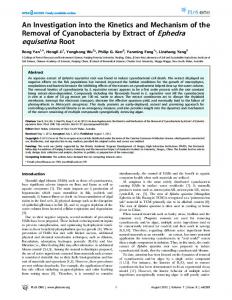
where wi is the ith root of f .x/. To design a neural network (i.e., feedforward neural network) model for nding the roots of polynomials, we expand the corresponding polynomial into an FNN, and use the FNN to express or approximate the polynomial so that the hidden-layer weights of the FNN represent the coefcients of the individual linear monomial factors such as 1 or x. As a result, a two-layered FNN model for nding roots of polynomials can be constructed, as shown in Figure 1. This model, which is somewhat similar to the 6 ¡ 5 neural network structure (Hormis, Antonion, & Mentzelopoulou, 1995), is in essence a onelayer linear network extended by a sum product (6 ¡ 5) unit. The network has two input nodes corresponding to the terms of 1 and x, n hidden nodes of forming the difference between the input x and the connection weights wi ’s, and one output product node that performs the multiplications on the outputs of the n hidden nodes. Only the weights between the input node that is clamped at value 1 and the hidden nodes need to be trained. The weights between the input x and the hidden nodes and those between the hidden nodes to the output node are always xed at 1. In mathematical terminology,

w1 1

w2

1

1

wn 1 1 wn 1

x

Figure 1: Feedforward neural network architecture for nding the roots of polynomials.

1724


the output corresponding to the ith hidden node can be represented as yi D x ¡ wi ¢ 1 D x ¡ wi

(1.3)

where wi .i D 1; 2; : : : ; n/ are the network weights (the roots of the polynomial). The output of the output layer performing multiplication on the outputs of the hidden layer can be written as O D y.x/

n Y iD1

yi D

n Y iD1

.x ¡ wi /:

(1.4)

The outer-supervised signal dened at the output of this network model is the polynomial f .x/. Here, this NRF structure is referred to as the 6 ¡ 5 model. In fact, equation 1.4 can be performed by means of the logarithmic operator. Thus, we can obtain the following equation: N O D ln jy.x/j D y.x/

n X iD1

ln jx ¡ wi j:

(1.5)

As a result, another NRF model, which is structurally similar to the factorization network model proposed by Perantonis, Ampazis, Varoufakis, and Antoniou (1998), can be easily derived. In this model, the resulting hidden nodes, which originally computed the linear differences (in other words, make the summation) between the input x and the connection weight w in the 6 ¡ 5 model, become nonlinear one with a logarithmic operator activation function, and the resulting output node performs a linear summation instead of multiplication. Therefore, this resulting NRF structure is referred to as the log 6 model (Huang, 2000). For such constructed NRFs, the corresponding training algorithm is generally the traditional backpropagation algorithm (BPA) with gradient-descent type, which has a very slow training speed and often leads to unsatisfactory solutions when training the network unless a suitably chosen set of initialized connection weights is given in advance (Huang, 2000). Although the initializing connection weights can be derived from separating different roots of polynomials by means of polynomial theory, it will still take a long time to achieve the upper and lower bounds of the roots of polynomials, especially for the higher-order polynomials (Huang, 2000; Huang & Chi, 2001). In order to alleviate this difculty, we adopt the idea of a constrained learning algorithm (CLA) rst proposed by Karras and Perantonis (1995) and incorporate the a priori information about the relationship between the roots (the connection weights) and the coefcients of a polynomial into the BPA. This facilitates the learning process and leads to better solutions. As a result, we have developed a CLA for nding the roots of a polynomial (Huang & Chi, 2001), which did speed up the convergent process and


1725

improve the accuracy for nding the roots of polynomials with respect to previous results (Huang, 2000). Specically, the key point to stress is that this CLA is not sensitive to the initial weights (roots). It was also observed that a large number of computations for this CLA are spent on computing the constrained relation, which is of computational complexity of the order O.2n / between roots and coefcients of polynomial and the corresponding derivatives. This problem will become more serious for very high-order polynomials. Therefore, a method that requires fewer computations of the constrained relation between roots and coefcients will signicantly reduce training time. In the light of the fundamental idea of the CLAs, a constrained learning method based on the constrained relation between the root moments (Stathaki & Constantinides, 1995; Stathaki, 1998; Stathaki & Fotinapoulos, 2001) and the coefcients of polynomial can be constructed to solve this problem. Indeed, we have proved that the corresponding computational complexity, which is of the order O.nm3 /, for the root moment method (RMM) is much lower than the root coefcient methods (RCM) (Huang, Chi, & Siu, 2000). As a result, we consider that the roots of high-order polynomials can be found by this approach. In this article, we present the constrained relation between the root moments and the coefcients of polynomial, derive the corresponding CLA, and compare the computational complexities of the RMM-based NRF (RMM-NRF) with the RCM-based NRF (RCM-NRF). It has been found that neural methods have a signicant advantage over nonneural methods like Muller and Laguerre in mathematica roots function and that the RMM-NRF is signicantly faster than the RCM-NRF. We then focus on discussing how to apply this new RMM-NRF to nd the arbitrary roots of arbitrary polynomials. We discuss and compare the performance of two specic structures of the NRFs: the 6 ¡ 5 and log 6 models. It was found that the total performance of the log 6 model is better than that of the 6 ¡ 5 model. Moreover, it was also found that there are seldom local minima with the NRFs on the error surface if all the a priori information from polynomials has been appropriately encoded into the CLA. In addition, to apply this CLA to solve practical problems more conveniently, we investigate the effects of the three controlling parameters with the CLA on the performance of the two NRFs. The simulation results show that the training speed improves as the values of the three controlling parameters increase, while the estimated root accuracies and variances are almost kept unchanged. Section 2 of this letter presents the constrained relation between the root moment and the coefcients of polynomials, and discusses and derives the corresponding constrained learning algorithm based on the root moments for nding the roots of polynomials. In section 3, the computational complexities for the two NRFs of the RMM and the RCM, as well as traditional methods, are discussed, and the performance of the neural root-nding method is compared to the nonneural method’s performance. Experimen-

1726


tal results are reported and discussed in section 4. Section 5 presents some concluding remarks. 2 Complex Constrained Learning Algorithm Based on Root Moments of Polynomial 2.1 The Root Moments of Polynomial. We have discussed the fundamental constrained relationship, referred to as the root coefcient relation, between the (real or complex) roots and the coefcients of polynomials, and formulated this relation into the conventional BPA to get the corresponding CLA for nding the roots of polynomials (Huang & Chi, 2001; Huang et al., 2003). It has been found that there exists another important well-known constrained relationship, referred to as root moment relation, between the roots and the root moments of polynomial rst formulated by Sir Isaac Newton; the resulting relationship is known as the Newton identity (Stathaki & Constantinides, 1995; Stathaki, 1998; Stathaki & Fotinopoulos, 2001). The concept for the root moment of polynomial is dened as follows: Denition 1. For an n-order polynomial described by equation 1.1, assume that the corresponding n roots are, respectively, w1 ; w2 ; : : : ; and wn . Then the m.m 2 Z/ order root moment of the polynomial is dened as m m Sm D wm 1 C w2 C ¢ ¢ ¢ C wn D

n X

wm i :

(2.1)

iD1

Obviously, Sm ’s are possibly complex numbers that depend on wi ’s. Furm thermore, there hold S0 D n and dS D mwm¡1 . i dwi According to this denition of root moment, a recursive relationship between the m-order root moment and the coefcients of polynomial can be obtained as follows. First, for the case of m ¸ 0, we have (Stathaki, 1998): 8 S1 C a 1 D 0 > > > > > > > > C C ¢ ¢ ¢ C D 0; · S a S ma .m n/ 1 m¡1 m > : m Sm C a1 Sm¡1 C ¢ ¢ ¢ C an Sm¡n D 0; .m > n/: Second, for the case of m < 0, we have: 8 > >an S¡1 C an¡1 D 0 > > > > > > a S C an¡1 SmC1 C ¢ ¢ ¢ C jmjanCm D 0; > : n m an Sm C an¡1 SmC1 C ¢ ¢ ¢ C SmCn D 0;

(2.3) .m ¸ ¡n; a0 D 1/ .m < ¡n/


1727

In fact, it can be proven that the two following formulas hold: Sm C a1 Sm¡1 C ¢ ¢ ¢ C an Sm¡n D 0;

.m > n/

(2a.2)

and an Sm C an¡1 SmC1 C ¢ ¢ ¢ C SmCn D 0;

.m < ¡n/:

(2a.3)

Consequently, for jmj > n (outside the polynomial coefcients window), we can obtain a unied recursive relation as follows: Sm C a1 Sm¡1 C ¢ ¢ ¢ C an Sm¡n D 0;

.jmj > n/

(2.4)

The recursive relationships in equations 2.2 and 2.3 are named as Newton identities. From these Newton identities, we can obtain a theorem as follows: Theorem 1. Suppose that an n-order polynomial described by equation 1.1 is known. Then a set of parameters (root moment) fSm ; m D 1; 2; : : : ; n/ can be uniquely determined recursively by equation 2.2. Conversely, given n root moments fSm ; m D 1; 2; : : : ; n/, an n-order polynomial described by equation 1.1 can be uniquely determined recursively by equation 2.2. For the case of m < 0, however, a theorem similar to the above conclusion can be stated as follows: Theorem 2. Suppose that an n-order polynomial described by equation 1.1 is known. Then a set of parameters (root moment) fSm ; m D ¡1; ¡2; : : : ; ¡n/ can be uniquely determined recursively by equation 2.3. Conversely, given n root moments fSm ; m D ¡1; ¡2; : : : ; ¡n/, an n-order polynomial described by equation 1.1 can be uniquely determined recursively by equation 2.3. In fact, we can also derive the root moment from the Cauchy residue theorem, which is dened as 1 Sm D 2¼j

I X n 0 iD1

1 zm dz; .z ¡ ri /

(2.5)

where 0 is a closed contour, dened as z D ½.µ /e jµ , and contains the roots of the required factor of f .z/. From equation 1.1, we have f 0 .z/ D

n X f .z/ : ¡ ri z iD1

(2.6)

1728


Hence, equation 2.5 can be rewritten as 1 Sm D 2¼j

I 0

f 0 .z/ m z dz: f .z/

(2.7)

From the above denition of the root moment, we have the following corollary: Corollary 1. The root moments of the product f .z/ D f1 .z/ f2 .z/ and the ratio f .z/ D f1 .z/=f2 .z/ can be respectively derived as: f .z/

Sm

f .z/ Sm

f .z/

D Sm1 D

f .z/ Sm1

f .z/

(2.8)

f .z/ Sm2

(2.9)

C Sm2 ¡

Moreover, we can derive another corollary about the gradual behaviors of the root moments as the order m becomes sufciently large or small as follows: Corollary 2. Assume that rmax and rmin are respectively the maximum and minimum modulus roots of f .z/. Then we can derive lim Sm D rm max

m!1

lim Sm D rm min

m!¡1

(2.10) (2.11)

That is, when m is sufciently large, the root rmax with the maximum modulus will dominate the sum Sm , while the root rmin with minimum modulus will dominate the sum Sm when m is sufciently small. In addition, it is very easy to derive another corollary about the reciprocal of the roots: Corollary 3. If a new polynomial is dened as g.z/ D zn f .z¡1 /, then it has reciprocal roots with the original polynomial f .z/. These corollaries and conclusions form the basis for using the root moments of polynomials to nd the roots of polynomials. In the following, we derive the corresponding complex CLA based on the root moments’ constrained relation (i.e., conditions) implicit in polynomials to train the NRFs for nding the arbitrary roots of arbitrary polynomials. 2.2 Complex Constrained Learning Algorithm for Finding the Arbitrary Roots of Arbitrary Polynomial. From Huang (2000), Huang et al. (2000), and Huang et al. (2003), it can be found that the root nding method based on the CLA is apparently faster than the simple BP learning rule based on careful selection of initial synaptic weights. Therefore, in the following, we deduce this CLA and extend it to a more general complex version.


1729

Suppose that there are P training patterns selected from the complex region jxj < 1. An error cost function (ECF) is dened at the output of the FNN root nder, E.w/ D

P P 1 X 1 X jep .w/j2 D jop ¡ yp j2 ; 2P pD1 2P pD1

(2.12)

where w is the set of all connection weights in the network model; op D f .xp / or Qnln f .xp / denotes Pn the target (outer-supervised) signal to be rooted; yp D iD1 .xp ¡ wi / or iD1 ln jx ¡ wi j represents the actual output of the network; and p D 1; 2; : : : ; P is an index labeling the training patterns. The above variables and functions are all possibly complex numbers, so in the following, the derivations according to the rule of complex variables must be observed. For an arbitrary complex variable, p z D xC iy, where x and y are the real and imaginary parts of z, and i D ¡1. For the convenience of deducing the following learning algorithm, we give a denition of the derivative of a real-valued function with respect to complex variable: Denition 2. Assume that a real-valued function U.w/ is the function of complex variable w with the real and imaginary parts w1 and w2 . Then the derivative D @U.w/ C i @U.w/ of U.w/ with respect to w is dened as @U.w/ @w @w1 @w2 . Consequently, the BPA based on the gradient descent can easily be deduced from the E.w/. By taking the partial derivative of E.w/ with respect to w, we can obtain Ji D

P n Y 1X @ E.w/ D ep .w/ ¢ .xp ¡ wj / @wi P pD1 j6Di

P xp ¡ wi 1X ep .w/ ¢ : jxp ¡ wi j2 P pD1

or

(2.13)

As a result, the BPA based on the gradient descent is described as follows: dw i D ¡´Ji

(2.14)

where dw i D wi .k/ ¡ wi .k ¡ 1/ denotes the difference between wi .k/ and wi .k ¡ 1/, the current and the past weights. According to the above formulated constrained conditions based on the root moments dened in equations 2.2 to 2.4, we can uniformly write them as 8 D 0;

(2.15)

1730


where 8 D [81 ; 82 ; : : : ; 8m ]T .m · n/ (T denotes the transpose of a vector or matrix) is a vector composed of the constraint conditions of any one of equations 2.2 to 2.4. By considering the ECF, which possibly contains many long, narrow troughs (Hush, Horne, & Salas, 1992), a constraint for updated connection weights is imposed in order to avoid missing the global minimum. Consequently, the sum of the squared absolute value of the individual weight changes takes a predetermined positive value .±P/2 (±P > 0 is a constant): n X iD1

jdwi j2 D .±P/2 :

(2.16)

This means that at each epoch, the search for an optimum new point in the weight space is restricted to a small hypersphere with radius ±P centered at the point dened by the current weight vector. If ±P is small enough, the change to E.w/ and to 8 induced by changes in the weights can be approximated by the rst differentials, dE.w/ and d8, respectively. In order to derive the corresponding CLA based on the constraint conditions of equations 2.2 or 2.3 and 2.16, assume that d8 is equal to a predetermined vector quantity ±Q, designed to bring 8 closer to its target (zero). The objective of the learning process is to ensure that the maximum possible change in jdE.w/j is achieved at each epoch. Usually the maximization of jdE.w/j can be carried out analytically by introducing suitable Lagrange multipliers. Thus, a vector V D [v1 ; v2 ; : : : ; vm ]T of Lagrange multipliers is needed to take into account the constraints in equation 2.15. Another Lagrange multiplier ¹ is introduced for equation 2.16. By introducing the function ", d" can be expanded as follows:

d" D

n X iD1

H

Ji dwi C .±Q ¡

n X

" dw i FH i /V

iD1 .j/

2

C ¹ .±P/ ¡

n X iD1

# 2

jdw i j

; (2.17)

@8

.2/ .m/ T j where Fi D [F.1/ i ; Fi ; : : : ; Fi ] , Fi D @wi .i D 1; 2; : : : ; n; j D 1; 2; : : : ; m/, · denotes the number of the constraint conditions in equation 2.15. m n Further, to maximize jd"j (in fact, minimize d") at each epoch, we demand that

d2 " D

n X iD1

2 .Ji ¡ FH i V ¡ 2¹dwi /d wi D 0

d3 " D ¡2¹

n X .d2 wi /2 < 0: iD1

(2.18)

(2.19)


1731

As a result, the coefcients of d2 wi in equation 2.18 should vanish, that is, Ji FH V ¡ i 2¹ 2¹

dw i D

(2.20)

where the values of Lagrange multipliers ¹ and V can beP readily evaluated from equations 2.16 and 2.20 and the condition .±QH ¡ niD1 dwi FH i /V D 0 is embodied in equation 2.15 with the following results: " 1 ¹D¡ 2

¡1 IJJ ¡ IH JF IFF I JF

#1=2

¡1 .±P/2 ¡ ±QH IFF ±Q

¡1 ¡1 V D ¡2¹IFF ±Q C IFF IJF ;

where IJJ D dened by .j/

IJF D

Pn

2 iD1 jJi j

n X iD1

(2.21) (2.22)

is a scalar and I JF is a vector whose components are

.j/

Ji Fi ; j D 1; 2; : : : ; m:

(2.23)

P jk .j/ Specically, IFF is a matrix, whose elements are dened by IFF D niD1 Fi F.k/ i .j; k D 1; 2; : : : ; m/. Obviously, there are .m C 1/ parameters ±P; ±Qj .j D 1; 2; : : : ; m/, which need to be set before the learning process begins. Parameter ±P is often adaptively selected as (Huang, 2001) µp

±P.t/ D ±P0 .1 ¡ e¡ t /; ±P.0/ D ±P 0 ;

(2.24)

where ±P0 is the initial value for ±P, which is usually chosen as a larger value, t > 0 is the time index for training, and µp is the scale coefcient of time index t, which is usually set as µp > 1. However, the vector parameters ±Qj .j D 1; 2; : : : ; m/ are generally selected as proportional to 8j , that is, ±Qj D ¡k8j (j D 1; 2; : : : ; m and k > 0), which ensures that the constraints 8 move toward zero at an exponential rate as training progresses. ¡1 From equation 2.19, we note that k should satisfy k · ±P.8H IFF 8/¡1=2 . q In practice, the simplest choice for k is k D ´±P= 8H I¡1 FF 8, where 0 < ´ < 1 is another free parameter of the algorithm but ±P. 3 Computational Complexity Estimates of the RMM-NRF and the RCM-NRF In this section, we compare the computational complexities of our proposed RM-based roots-nding method with the original RC-based roots-nding

1732


method, as well as traditional root nders such as Muller and Laguerre (William et al., 1992; Anthony & Philip, 1978), and show theoretically and experimentally that the speed of this RMM-RNF is signicantly faster than the RCM-NRF and those traditional root nders. It can be seen from the CLA that at each iterative epoch, we have to compute the values of the constraint conditions of 8 and their derivatives, @8=@w, which are sharply dominant in all CLA computations (multiplication or division operations). In order to estimate the computational complexity of the multiplication or division operations for the RMM, we can, from the constraint conditions of equation 2.23, achieve @8=@w D [F.1/ ; F.2/ ; : : : ; F.n/ ]T as follows: 8 .1/ F D [1; 1; : : : ; 1]T > > > .2/ T > > > > >F.n/ D [n¸n¡1 C .n ¡ 1/a1 ¸n¡2 C ¢ ¢ ¢ C an¡1 ; n¸n¡1 C ¢¢¢ > 1 1 2 : n¡1 C an¡1 ; : : : ; n¸n C .n ¡ 1/a1 ¸n¡2 C ¢ ¢ ¢ C an¡1 ]T : n

(3.1)

Consequently, we can estimate the number of multiplication operations at each epoch for computing the constraint conditions of equation 2.2 for 8 and their derivatives @ 8=@w, stated in the following remark (Huang et al., 2000; Huang, 2004): 1 Remark 1. At each epoch for nding the complex roots of a given arbitrary polynomial f .x/ of order n based on the constrained learning neural networks using the m constraint conditions ordered from the rst one of equation 2.2, the estimate of the number of multiplication operations needed for computing 8 and @8=@w, CERMM .n; m/, is CERMM.n; m/ D

2 .m ¡ 1/.nm2 C 10nm C 3m ¡ 12n C 6/: 3

(3.2)

Obviously, CERMM.n/ is of the order O.nm3 / multiplication operations. Specically, when m D n, equation 3.2 becomes CES .n; n/ D 23 .n ¡ 1/.n3 C 10n2 ¡ 9n C 6/. In addition, for the RCM, we can obtain @ 8=@w D [F.1/ ; F.2/ ; : : : ; F.m/ ]T from the constraint condition of the relation between the roots and coef-

1 Here, the most general case for complex computations, which have four times the real computations, is considered.


1733

cients of the polynomial (see, Huang, 2000) as follows: 8 .1/ F D [1; 1; : : : ; 1]T > > " #T > > n n n > X X X > .2/ > > F D wi ; wi ; : : : ; wi > > < i6D1

i6D2

i6Dn

i6D1

i6D2

i6Dn

(3.3)

:: > > : > > " #T > > m m m Y Y Y > > .m/ > wi ; wi ; : : : ; wi : > :F D

As a result, the estimate of the number of multiplication operations at each epoch for a given polynomial f .x/ of order n is stated as follows (Huang et al., 2000; Huang, in press): Remark 2. At each epoch for nding the complex roots of a given arbitrary polynomial f .x/ of order n based on the constrained learning neural networks using the m constraint conditions ordered from the rst one of equation 3.3, the estimate of the number of multiplication operations needed for computing 8 and @8=@w, CERCM.n; m/, is: 0 1 m m m X X X j j j 2 CERCM .n; m/ D 4 @ j Cn ¡ jCn ¡ Cn C n C 1A : jD0

jD0

(3.4)

jD0

2 Obviously, CERCM.n/ is of the order O.Cm n m / multiplication operations, which is considerably higher than that of the RMM. Specically, when m D n, equation 3.4 becomes CERCM .n; n/ D 4[.n2 ¡n¡4/2n¡2 CnC1]. Obviously, CERCM.n; n/ is of the order O.2n / multiplication operations. CERCM .n;n/ If we dene a ratio, rc , of CERCM .n; n/ and CERMM.n; n/; rc D CE , RMM .n;n/ then it can be readily deduced that

lim rc D lim

n!1

n!1

CERCM .n; n/ D 1: CERMM.n; n/

(3.5)

Table 1 gives the comparisons between the computational complexities of the RCM-NRF and the RMM-NRF versus the polynomial order n. From the results, it is easily found that the RMM-NRF has less computational cost as n increases. However, when n is chosen as a smaller value (e.g., n · 5), the conclusion is the opposite. Therefore, it is for higher-order polynomials that the RMM-NRF exhibits its strong potential in computational complexity. In addition, the computational complexities for those traditional root nders in mathematica roots function such as Muller and Laguerre (Mourrain, Pan, & Ruatta, 2003; Milovanovic & Petkovic, 1986) are generally of the order O.3n /,

1734


Table 1: Comparisons of Computational Complexities of the Original RCM and the RMM. n

1

2

3

4

5

6

7

8

9

10

11

12

CERCM .n/ 0 4 32 148 536 1692 4896 13,348 34,856 88,108 217,136 524,340 CERMM .n/ 0 24 128 388 896 1760 3104 5068 7808 11,496 16,320 22,484

while the computational complexity for the fastest method, like JenkinsTraub, is only of the order over O.n4 /. It is substantially higher than our proposed RMM, especially our derived recursive RMM (see Huang, 2004). To further verify the correctness of these theoretical analyses, we take a seven-order polynomial— f .x/ D x7 C .1:2 ¡ 0:5i/x6 C .¡6:5 C 1:4i/x4 C 2:93ix2 C .1:7 C 2:4i/x C 2:4 ¡ 0:3i, for example—to compare the performance of the RCM-NRF and the RMM-NRF. Here, we consider only the case of the log 6 model. Assume that the controlling parameters with the CLA for two methods are both selected as ±P0 D 2:0, µp D 5:0, and ´ D 0:6, and let the termination error be er D 1:0 £ 10¡8 . The training sample pairs .x; f .x// are obtained from the complex domain of jxj < 1, where the total training sample number P is xed as 100. In the experiment, assume that we adopt Pentium III with a CPU clock of 795 Mhz and RAM of 256 Mb, and use Visual Fortran 90 to encode. After the NRFs respectively trained by these two methods converge, it was found that the RCM-NRF and the RMM-NRF take, respectively, 9196 and 2783 iterations, where the CPU times taken by the former and the latter are 277 seconds and 41 seconds. That is, the training speed of the RMM is almost seven times that of the RCM, which completely supports our theoretical analyses. Figure 2 depicts the two learning error curves (LEC) of the two methods, and Figure 3 shows the LEC for the BPA-based NRF in the case of the learning coefcient ´ D 0:1. From Figures 2 and 3, it can be seen that the two CLAs are signicantly faster than the BPA, and the RMM-based CLA is essentially faster than the RCM-based CLA. In addition, we use the same parameters as above but with the termination accuracy er D 1:0 £ 10¡25 to compare the performance of the RCM-NRF and the RMM-NRF, as well as the two nonneural methods of Muller and Laguerre. Here, the important point is that Muller’s and Laguerre’s methods are also encoded by Visual Fortran 90 to perform the roots-nding program according to formulas of 9.5.2 and 9.5.3 and 9.5.4 to 9.5.11 in William et al. (1992), respectively. Moreover, to statistically evaluate different root nders, the experiments were repeated 10 times with different initial weight values from the uniform distribution in [¡1; 1] (for the two nonneural methods of Muller and Laguerre, the initial roots are determined by polynomial theory; Huang, 2000, 2004). Consequently, the average iterating numbers, the average CPU times, and the average estimated variances for the four methods


1735

Figure 2: Learning error curves of the original RCM-NRF and the RMM-NRF for a seven-order polynomial.

Figure 3: Learning error curve for the BPA–based NRF in the case of the learning coefcient ´ D 0:1 for a seven-order polynomial.

1736


Table 2: Statistical Performance Comparisons of the Original RCM-NRF and the RMM-NRF for a Seven-Order Polynomial f .x/.

Indices

Average Iterating Numbers

Average CPU Times (seconds)

Average Estimated Variances

RMM RCM Muller Laguerre

23,242 276,425 519,374 432,463

972.4 1207.2 2542.2 2312.4

3.26367E¡026 2.32545E¡026 1.32443E¡026 4.23151E¡026

Figure 4: Histogram comparisons among the iterating numbers for four rootnding methods.

are respectively shown in Table 2, and the corresponding histograms for the average iterating numbers and the average CPU times are respectively illustrated in Figures 4 and 5. Table 2 shows that the RMM-NRF is signicantly faster than the RCMNRF, and that the two NRFs are also faster than the two nonneural methods. Moreover, the accuracies and the CPU times consumed for the two neural approaches are higher and shorter than the ones for the two nonneural methods. This is because Muller’s and Laguerre’s methods iteratively ob-


1737

Figure 5: Histogram comparisons among the CPU times consumed for four root-nding methods.

tain one root at a time so that the accuracy for the reduced polynomial is affected, which will result in lower root accuracies and longer iterating times (including the times of carefully selecting initial root values).

Comments. Why do we revisit this topic of the root-nding polynomial since there have been many numerical methods? The other motivation except for the parallel processing fact for neural methods includes that the neural methods can simultaneously nd all roots, while the traditional numerical methods can sequentially nd the roots only by the deation method so that each new root is known with only nite accuracy, and errors will creep into the determination of the coefcients of the successively deated polynomial (William et al., 1992). Hence, the accuracy for the nonneural numerical method is fundamentally limited and cannot surpass the one for the neural root-nding method. In addition, all nonneural methods need to nd good candidates with initial root values; otherwise, the designed root nder will not converge (William et al., 1992), which will increase computational complexity and consume additional processing time. On the other hand, our proposed neural approaches are instructed by the a priori information from the polynomials imposed into the CLA so that they almost do not need to compute any initial root values except for randomly selecting them from the uniform distribution in [¡1; 1].

1738


Considering these points, we shall focus on the RMM-NRF in presenting and discussing experimental results. 4 Experimental Results and Discussions In order to verify the effectiveness and efciency of our proposed approaches, we conducted several experiments. We make two assumptions in the following experiments. First, for each polynomial involved f .x/, the input training sample pairs .x; f .x// are obtained from the complex domain of jxj < 1, and the total number, P, of input training sample pairs is xed at 100. Second, the initial weight (root) values of the FNNRF are randomly selected from the uniform distribution in [¡1; 1]. 4.1 Polynomial with Known Roots. There is a six-order test polynomial f1 .x/ with known complex roots generated from ri D 0:9£ exp.j ¼3i /.i D 1; 2; : : : ; 6/, the roots distributions of which are shown in Figure 6. We use an FNNRF with a 2-6-1 structure to nd the roots of this polynomial. Assume that three controlling parameters with the CLA are chosen as ±P 0 D 10:0, µp D 10:0, and ´ D 0:3, which are kept unchanged in this example, and that three termination errors of er D 0:1, er D 0:01, and er D 0:001 are respectively considered. To evaluate the statistical performance of the NRFs, for each case, we conducted 30 repeating experiments by choosing different initial connection weights from the uniform distribution in [¡1; 1] to

1.2 1 0.8 0.6 0.4 0.2 0 -0.2 -0.4 -0.6 -0.8 -1 -1.2 -1.2 -1 -0.8 -0.6 -0.4 -0.2

0

0.2 0.4 0.6 0.8

Figure 6: Roots distributions of f1 .x/ in the complex plane.

1

1.2


1739

observe the experimental results for the 6 ¡ 5 and log 6 models. After the corresponding FNNRFs were trained by the CLA to converge to the given accuracies, the estimated convergent roots corresponding to the two models are respectively depicted in Figures 7 through 9, where the true roots are represented by the bigger black dots. Figures 7 to 9 show that the estimated root accuracies get higher and higher, and the scatters for the estimated roots become smaller and smaller as the termination error increases. Figure 7 shows that for the termination error case of er D 0:1, the accuracy for the 6 ¡ 5 model is obviously higher than the one for the log 6 model. The reason is that the logarithmic operator used in the log 6 model primarily plays a role of transformation, compressing a larger numerical value into a smaller one. Thus, the termination error er D 0:1 in the log 6 model is to a certain extent equivalent to er D e0:1 in the 6 ¡ 5 model. Therefore, it is the lower training accuracy that has resulted in the poor estimated root accuracy. The same conclusions hold for the other two termination error cases; however, the differences between the two models as the training accuracy increases (i.e, the termination error decreases) are not great (see Figures 8 and 9). At the same time, this phenomenon also indirectly shows that the FNNRF based on root moments results in a very fast convergent speed. In addition, assume that the termination error is xed at er D 1:0 £ 10¡9 . We repeat the 30 experiments to get the average estimated roots (including the average estimated variances), the average iterating numbers, the average CPU times, and the average relative estimate errors (dr ), as shown in Table 3.2 From Table 3, it can be seen that from the statistical sense, the 6 ¡ 5 model is of higher estimated accuracy than the log 6 one, but the latter has a shorter training time than the former: the average CPU time for the 6 ¡ 5 model is 52 seconds longer than that for the log 6 one. The reason is also due to the compressing transformation of the log 6 model. Figures 10 and 11 show, respectively, two sets of logarithmic learning root curves of the two models for one of 30 experiments, where the logarithmic operations of the iterating numbers are done in order to show the magnied starting parts of the curves. For each plot, there are 12 curves representing the real and imaginary parts of the six complex roots for some NRF (in fact, we can get the six complex roots only by means of the NRF). From Figures 10 and 11, it can be seen that the 6 ¡ 5 model yields drastic uctuations around their true (estimated) root values, which may result in many long, 2

The average relative estimate error is dened as

dr D

K n .k/ 1 1 XX xi ¡ xO i ¢ xi K n kD1

i

where K is the repeated experimental number, xi is the ith true (exact) root value of the given polynomial, and xO .k/ i is the kth estimated value of the ith root (i.e., the weight, wi ).

1740

D.-S. Huang, H. Ip. and Z. Chi 1.2 1 0.8 0.6 0.4 0.2 0 -0.2 -0.4 -0.6 -0.8 -1 -1.2 -1.2 -1 -0.8 -0.6 -0.4 -0.2

0

(a) er

0.2 0.4 0.6 0.8

1

1.2

1

1.2

0.1

1.2 1 0.8 0.6 0.4 0.2 0 -0.2 -0.4 -0.6 -0.8 -1 -1.2 -1.2 -1 -0.8 -0.6 -0.4 -0.2

0

(b) er

0.2 0.4 0.6 0.8

0.1

Figure 7: Estimated roots distributions of f1 .x/ in the complex plane for the 6 ¡ 5 and log 6 models in the case of er D 0:1. (a) 6 ¡ 5 model. (b) log 6 model.


1741

1.2 1 0.8 0.6 0.4 0.2 0 -0.2 -0.4 -0.6 -0.8 -1 -1.2 -1.2 -1 -0.8 -0.6 -0.4 -0.2

0

(a) er

0.2 0.4 0.6 0.8

1

1.2

1

1.2

0.01

1.2 1 0.8 0.6 0.4 0.2 0 -0.2 -0.4 -0.6 -0.8 -1 -1.2 -1.2 -1 -0.8 -0.6 -0.4 -0.2

0

(b) er

0.2 0.4 0.6 0.8

0.01

Figure 8: Estimated roots distributions in the complex plane of f1 .x/ for the 6 ¡ 5 and log 6 models in the case of er D 0:01. (a) 6 ¡ 5 model. (b) log 6 model.

1742

D.-S. Huang, H. Ip. and Z. Chi 1.2 1 0.8 0.6 0.4 0.2 0 -0.2 -0.4 -0.6 -0.8 -1 -1.2 -1.2 -1 -0.8 -0.6 -0.4 -0.2

0

(a) er

0.2 0.4 0.6 0.8

1

1.2

1

1.2

0.001

1.2 1 0.8 0.6 0.4 0.2 0 -0.2 -0.4 -0.6 -0.8 -1 -1.2 -1.2 -1 -0.8 -0.6 -0.4 -0.2

(b) er

0

0.2 0.4 0.6 0.8

0.001



1743

Table 3: Statistical Performance Comparison of the 6 ¡5– and the Log 6–Based FNNRF Models for f1 .x/. Average Estimated Roots (±P0 D 10:0; µp D 10:0; ´ D 0:3) Indices Average estimated roots

w1 w2 w3 w4 w5 w6

Average iterating number Average CPU times (seconds) Average relative estimated error (dr ) Average estimated variance

log 6 Model

6 ¡ 5 Model

(0.8999990, 1.3729134E¡06) (¡0.8999991, ¡1.1557200E¡07) (0.4499939, 0.7794214) (¡0.4500013, ¡0.7794217) (¡0.4499971, 0.7794194) (0.4499970, ¡0.7794210)

(0.8999987, ¡4.1471349E¡06) (¡0.9000001, ¡8.5237025E¡07) (0.4499981, 0.7794229) (¡0.4499988, ¡0.7794209) (¡0.4499974, 0.7794240) (0.4499984, ¡0.7794222)

137,541

226,690

118.24

170.33

1.133025533350818E¡005

8.708582759808792E¡006

2.706395396765315E¡005

2.147191933435669E¡005

Figure 10: The 12 learning weights (roots) curves of f1 .x/ for the 6 ¡ 5 model versus the logarithmic iterating numbers.

1744


Figure 11: The 12 learning weights (roots) curves of f1 .x/ for the log 6 model versus the logarithmic iterating numbers.

narrow troughs that are at in one direction and steep in other directions. This phenomenon slowed the corresponding training speed signicantly. In contrast, the log 6 model is capable of compressing the input dynamic range so that it can produce a smoother cost function landscape, avoiding deep valleys and thus facilitating learning. Therefore, for practical problems, the log 6 model is preferred. 4.2 Arbitrary Polynomial with Unknown Roots. To verify the efciency and effectiveness of this NRF based on the root moments of a polynomial, a nine-order arbitrary polynomial f2 .x/ D x9 C 2:1ix7 C 1:1x6 C .1:3 ¡ i/x3 C .1:4 C 0:6i/x C 5:3i is given to test the performance of the NRF. For this problem, an FNNRF with the structure of 2-9-1 is constructed to nd the roots of the polynomial. Assume that three controlling parameters with the CLA are respectively chosen as ±P0 D 8:0, µp D 5:0, and ´ D 0:4, which are also kept unchanged. And for three given sets of termination errors of er D 0:1, er D 0:01, and er D 0:001, we respectively conduct 30 repeating experiments by choosing different initial connection weights from the uniform distribution in [¡1; 1] to evaluate the statistical performance of the two NRFs. After the NRF converges, the estimated convergent roots corresponding to the two models are respectively depicted in complex planes, as shown in Figures 12 to 14, where only one root is inside the unit circle of the complex plane. These three gures show that similar phenomena can be observed for the experimental cases.


1745

1.5

1

0.5

0

-0.5

-1

-1.5 -1.5

-1

-0.5

0

(a) er

0.5

1

1.5

0.5

1

1.5

0.1

1.5

1

0.5

0

-0.5

-1

-1.5 -1.5

-1

-0.5

0

(b) er

0 .1

Figure 12: Estimated roots distributions in the complex plane of f2 .x/ for the 6 ¡ 5 and log 6 models in the case of er ¡ 0:1. (a) 6 ¡ 5 model. (b) log 6 model.

1746

D.-S. Huang, H. Ip. and Z. Chi 1.5

1

0.5

0

-0.5

-1

-1.5 -1.5

-1

-0.5

0

(a) er

0.5

1

1.5

0.5

1

1.5

0.01

1.5

1

0.5

0

-0.5

-1

-1.5 -1.5

-1

-0.5

0

(b) er

0.01



1747

1.5

1

0.5

0

-0.5

-1

-1.5 -1.5

-1

-0.5

0

(a) er

0.5

1

1.5

0.5

1

1.5

0.001

1.5

1

0.5

0

-0.5

-1

-1.5 -1.5

-1

-0.5

0

(b) er

0.001


1748


Here, the point that we must stress is that it has been found in experiments that for some initial connection weights, the 6 ¡ 5 model always oscillates around some local minimum. That is, there are possibly some local minima in the error surface of the 6 ¡ 5 model. Similarly, let er D 1:0 £ 10¡9 . We repeat the 30 experiments to get the average estimated roots (including the average estimated variances), the average reconstructed polynomial coefcients, the average iterating numbers, the average CPU times, and the average estimate accuracies3 (Cp ), as shown in Table 4. From Table 4, it can again be observed that from the statistical sense, the log 6 model has a faster training speed than the 6 ¡ 5 model, but the latter is of higher estimated accuracy than the former. In addition, Figures 15 and 16 illustrate respectively two sets of logarithmic learning weights (roots) curves of the two models for only one of 30 repeated experiments with identical initial connection weight values, where there are, for each subplot, two curves representing the real (the solid line) and imaginary (the dashed line) parts of one complex root. From Figures 15 and 16, it can be seen that the 6 ¡ 5 model is of slower convergent speed than the log 6 model, and the corresponding uctuation surrounding their true (estimated) root values is slightly conspicuous with respect to the latter. In addition, for some initial connection weights, we again found that there are oscillations surrounding certain local minima occurring in the process of searching the solutions. Therefore, it is again suggested that in applying this NRF to solving those practical problems, the log 6 model should be preferred to the direct 6 ¡ 5 model. 4.3 Effects of the Parameters with the CLA on the Performance of the NRFs. In order for the CLAs to be more conveniently applied to solving root-nding problems in practice, we investigate the effects of the three controlling parameters with the CLA on the performance of the NRFs. Assume that an arbitrary ve-order test polynomial with unknown roots f3 .x/ D x5 C 2:2x4 C .¡3:1 ¡ 0:5i/x3 C .2:4 ¡ 1:7i/x2 C 4:3ix C 2:35 ¡ 1:23i is given; we build an FNNRF with the structure of 2-5-1 to discuss the effects of the three controlling parameters used in the CLA, f±P0 ; µp ; ´g, on the performance of this NRF. In the following experiments, we always suppose that the termination error is xed at er D 1 £ 10¡8 for all cases, three sets of different values for each parameter of f±P0 ; µp ; ´g with the CLA are 3

The average estimate accuracy is dened as

Cp D

K n 1 1 XX ¢ jai ¡ aO .k/ i j; K n kD1 iD1

where K is the repeated experimental number, fai g is the coefcient of the polynomial, and aO .k/ i is the ith reconstructed polynomial coefcient value of the kth experiment.


1749

Table 4: Statistical Performance Comparison of the 6 ¡ 5– and Log 6–Based FNNRF Models for f2 .x/. Average Estimated Roots (±P0 D 8:0; µp D 5:0; ´ D 0:4) Indices Average estimated roots

w1 w2 w3 w4 w5 w6 w7 w8 w9

Average reconstructed polynomial coefcients

aN 1 aN 2 aN 3 aN 4 aN 5 aN 6 aN 7 aN 8 aN 9

Average iterating number Average CPU times (seconds) Average estimated accuracy .Cp / Average estimated variance

log 6 Model

6 ¡ 5 Model

(¡1.138758, ¡0.1249457) (0.9814540, ¡0.3930945) (1.029028, 0.5315055) (¡0.6140527, ¡0.7163082) (0.2785297, 1.157246) (¡0.5205935, 1.071421) (¡1.275355, 0.8272572) (1.105366, ¡1.250805) (0.1543829, ¡1.102276)

(¡1.138757, ¡0.1249474) (0.9814527, ¡0.3930941) (1.029029, 0.5315061) (¡0.6140542, ¡0.7163094) (0.2785297, 1.157247) (¡0.5205949, 1.071422) (¡1.275356, 0.8272576) (1.105367, ¡1.250804) (0.1543843, ¡1.102277)

234,239

267,529

135.16

278.54

5.855524581083182E¡005

8.679319172366640E¡006

2.164147025607199E¡005

3.248978567496603E¡006

(¡1.3808409E¡6, 1.0450681E¡6) (6.6061808E¡8, 1.0728835E¡7) (¡3.4644756E¡06, 2.100000) (¡2.8174892E¡07, 2.100000) (1.100003, ¡4.3437631E¡06) (1.100000, ¡1.0875538E¡06) (¡9.9966510E¡6, ¡5.5188639E¡6) (¡4.694555E¡9, 1.4712518E¡6) (2.8562122E¡6, 5.2243431E¡6) (1.5409139E¡6, 1.7070481E¡6) (1.299983, ¡1.000008) (1.300000, ¡0.9999995) (¡1.1211086E¡5, 2.4979285E¡5) (2.8605293E¡6, 1.9240313E¡6) (1.399990, 0.6000041) (1.399996, 0.6000024) (2.6458512E¡5, 5.299979) (6.8408231E¡6, 5.300003)

in turn chosen while keeping other two parameters unchanged, and for each case, we conduct 30 repeating experiments by choosing different initial connection weights from the uniform distribution in [¡1; 1] to evaluate the statistical performance of the two NRFs. 4.3.1 Case 1. The parameters µp D 5:0 and ´ D 0:5 remain unchanged, while ±P0 is respectively chosen as 15.0, 27.0, and 39.0. For this case, we design the corresponding CLA with these chosen parameters to train the two FNNRFs with 30 different initial weight values until the termination error is reached. Table 5 lists the average estimated roots (including the average estimated variances), the average reconstructed polynomial coefcients, the average iterating numbers, and the average estimate accuracies (Cp ). From Table 5, it can be seen that the iterating number (or the training time) becomes bigger and bigger (longer and longer) as the parameter ±P0 increases.

6¡5 model

log 6 model w1 w2 w3 w4 w5 aN 1 aN 2 aN 3 aN 4 aN 5

w1 w2 w3 w4 w5 aN 1 aN 2 aN 3 aN 4 aN 5



Average estimated roots




Indices

(2.199999, 5.1061312E¡7) (¡3.100002, ¡0.4999993) (2.400008, ¡1.700007) (2.6580785E¡5, 4.300016) (2.349960, ¡1.229988) 72,072 24.05 3.894946050153614E¡5 1.953243868591304E¡5

47,069 13.8 4.174685119040511E¡5 2.109834543554335E¡5

1.348195988200199E¡4

1.215649799242255E¡4

(2.200001, ¡3.5464765E-7) (¡3.099993, ¡0.4999999) (2.400001, ¡1.700003) (5.4543507E¡6, 4.300003) (2.350020, ¡1.230003)

2.434911676528762E¡4

2.408975763542598E¡4

(7.2838880E¡2, 0.4975683) (0.7840892, 0.9237731) (¡0.6682807, ¡0.9142268) (0.9756432, ¡0.5939271) (¡3.364290, 8.6812273E¡2)

18.21

12.76

(7.2835609E¡2, 0.4975790) (0.7840912, 0.9237689) (¡0.6682819, ¡0.9142306) (0.9756438, ¡0.5939294) (¡3.364290, 8.6812407E¡2)

50,755

28,398

2.039519060620054E¡5

3.940120231216149E¡5

25.88

104,382

(2.200002, ¡1.025199E¡6) (¡3.099999, ¡0.5000008) (2.399997, ¡1.700003) (2.0472218E¡5, 4.300006) (2.350006, ¡1.229997)

(7.283525E¡2, 0.4975761) (0.7840918, 0.9237698) (¡0.6682822, ¡0.9142287) (0.9756443, ¡0.5939285) (¡3.364291, 8.6812563E¡2)

1.317036301803572E¡4

2.560353167176954E¡4

22.34

66,752

(2.200003, 3.0497714E¡7) (¡3.100013, ¡0.5000228) (2.399964, ¡1.700022) (1.3247265E¡4, 4.300088) (2.349868, ¡1.230084)

(2.200001, ¡9.7428756E¡7) (¡3.100002, ¡0.5000318) (2.400039, ¡1.700037) (5.6860819E¡5, 4.300084) (2.350065, ¡1.230010)

(2.199985, 3.0177337E¡6) (¡3.099978, ¡0.5000005) (2.400114, ¡1.699990) (¡7.6231045E¡6, 4.300166) (2.349878, ¡1.230064)

±P0 D 39:0 .´ D 0:5; µp D 5:0/ (7.2854005E¡2, 0.497559) (0.7840888, 0.9237748) (¡0.6682967, ¡0.9142174) (0.9756408, ¡0.5939273) (¡3.36429, 8.6810604E¡2)

±P0 D 27:0 .´ D 0:5; µp D 5:0/ (7.2831228E¡2, 0.497575) (0.7841018, 0.9237837) (¡0.6682878, ¡0.9142339) (0.9756468, ¡0.5939333) (¡3.364293, 8.6809404E¡2)

(7.286707E¡2, 0.4975542) (0.7840687, 0.9237923) (¡0.6682831, ¡0.9142303) (0.9756445, ¡0.5939322) (¡3.364282, 8.6812876E¡2)

±P0 D 15:0 .´ D 0:5; µp D 5:0/

Table 5: Performance Comparisons Based on the Test Polynomial f3 .x/ Between the 6 ¡ 5 and Log 6 Models Under the Conditions of µp D 5:0 and ´ D 0:5 and ±P0 D 15:0; 27:0; 39:0.

1750 D.-S. Huang, H. Ip. and Z. Chi


1751

Figure 15: Logarithmic learning weights (roots) curves of the 6 ¡ 5 model for f2 .x/ versus the logarithmic iterating numbers: (a) w1 . (b) w2 . (c) w3 . (d) w4 . (e) w5 . (f) w6 . (g) w7 . (h) w8 . (i) w9 .

Moreover, it can be observed that from the statistical sense, the log 6 model has a faster training speed than the 6 ¡5 model, but the latter is of higher estimated accuracy than the former due to a longer training time. In addition, Figure 17 shows the logarithmic learning error curves for the two models in the case of three different ±P0 ’s for only one trial. Figure 17 shows that the convergent speed becomes slower and slower (i.e., the iterating number becomes bigger and bigger) as ±P0 increases. This phenomenon might be explained from the particulars of the CLA. In fact, from equation 2.20,

1752


Figure 16: Logarithmic learning weights (roots) curves of the log 6 model for f2 .x/ versus the logarithmic iterating numbers: (a) w1 . (b) w2 . (c) w3 . (d) w4 . (e) w5 . (f) w6 . (g) w7 . (h) w8 . (i) w9 .

q ¡1 ¡1 ±Qj D ¡´8j ±P= 8H IFF 8 and » D IJJ ¡ IH JF IFF I JF ¸ 0, we can follow: ¹D¡

1 » ¢p : 2±P 1 ¡ ´2

(4.1)

¡1 It can be derived that when ¹ ! 0 equation 2.21 approaches V ¼ IFF IJF ; then equation 2.19 can be rewritten as

dw i ¼

¡1 Ji ¡ F H i IFF I JF ; 2¹

(4.2)


1753

Figure 17: Logarithmic learning error curves for the (a) 6 ¡ 5 and (b) log 6 models under the conditions of µp D 5:0 and ´ D 0:5 and ±P0 D 15:0; 27:0; 39:0 for only one trial.

1754


which is more similar to the gradient descent formula of the BPA apart from ¡1 the second term ¡FH i IFF I JF =2¹ related to the a priori information of the root¡1 nding problem. When ¹ ! 1 equation 2.21 becomes V ¼ ¡2¹IFF ±Q; equation 2.19 can then be rewritten as ¡1 dw i ¼ FH i IFF ±Q;

(4.3)

which is more dependent on the a priori information of the problem at hand. Therefore, when ±P0 dynamically increases, from equation 4.1, ¹ becomes smaller and smaller so that the iterating for the connection weights switches to the gradient descent searching described in equation 4.2. Owing to ±P.t/ being adaptively chosen by equation 2.24, there is a longer training time for the bigger ±P0 before the iterating for the connection weights switches to the a priori information searching described in equation 4.3. Consequently, the convergent speed will certainly become slower for the bigger ±P0 , which shows that our experimental results are completely consistent with our theoretic analysis. In addition, from Figure 17, it can be seen that the uctuation for the 6 ¡ 5 model is much more drastic than the log 6 model, which is also consistent with the previous analyses. 4.3.2 Case 2. The parameters ±P0 D 12:0 and µp D 10:0 are kept unchanged, while ´ is respectively chosen as 0.4, 0.6, and 0.8. We design the corresponding CLA with these chosen parameters to train the two NRFs with 30 different initial weight values until the termination error is reached. Table 6 shows the average estimated roots (including the average estimated variances), the average reconstructed polynomial coefcients, the average iterating numbers, and the average estimate accuracies (Cp ). From Table 6, it can be observed that the iterating number increases as the parameter ´ increases. Moreover, it can be seen that from the statistical sense, the 6 ¡ 5 model has a slower training speed than the log 6 model, but the former is of higher estimated accuracy than the latter. Figure 18 shows the logarithmic learning error curves for the two models in the case of three different ´’s for only one trial. From this gure, it can be seen that the convergent speed becomes slower and slower as the parameter ´ increases. This phenomenon can be explained as follows: Since ±P.t/ is adaptively chosen by equation 2.24, the learning process always starts from ¹ ! 0 (the gradient-descent-based phase) to ¹ ! 1 (the a priori information-based searching phase). If ´.0 < ´ < 1/ is chosen as a bigger value, from equation 4.1, ¹ also becomes bigger. As a result, the role of ´ is dominant in the gradient-descent-based phase so that the bigger ´ will result in a slower searching process in the error surface. On the other hand, when the learning processing switches to the a priori information-based searching phase, the role of ±P.t/ becomes dominant. Obviously, during this phase, the

6¡5 model









Indices

2.679815124170259E¡4 1.385519662459264E¡4

2.554318324064775E¡4 1.410293537507154E¡4

(2.200001, 6.1516954E¡7) (¡3.099996, ¡0.5000052) (2.400009, ¡1.700007) (1.1644424E¡5, 4.300018) (2.349983, ¡1.229999) 72,083 21.37 4.134208802647477E¡5 2.230266509128565E¡005

(2.200000, 5.3594511E¡7) (¡3.100001, ¡0.4999996) (2.400007, ¡1.699998) (1.4605153E¡5, 4.300022) (2.349977, ¡1.230004) 47,582 15.82 4.232391613533809E¡5 2.176448291144487E¡005

(7.2838947E¡2, 0.4975726) (0.7840895, 0.9237724) (¡0.6682820, ¡0.9142290) (0.9756428, ¡0.5939277) (¡3.364291, 8.6811036E¡2)

12.57

9.45

(7.2840475E¡2, 0.4975722) (0.7840880, 0.9237713) (¡0.6682820, ¡0.9142277) (0.9756443, ¡0.5939280) (¡3.364291, 8.6811766E¡2)

50,025

30,594

2.261178583488332E¡005

4.376189929594654E¡5

27.55

101,549

(2.199999, ¡1.1945770E-7) (¡3.100004, ¡0.4999988) (2.400000, ¡1.700007) (1.1297192E¡5, 4.300014) (2.349992, ¡1.229999)

(7.2837636E¡2, 0.4975743) (0.7840908, 0.9237695) (¡0.6682816, ¡0.9142290) (0.9756443, ¡0.5939274) (¡3.364291, 8.6812787E¡2)

1.268341660759528E¡4

2.489754259489135E¡4

15.73

59,575

(2.200000, ¡6.7576769E¡7) (¡3.100017, ¡0.5000157) (2.400007, ¡1.700022) (1.0601872E¡4, 4.300101) (2.349869, ¡1.230183)

(2.199995, ¡2.2557870E¡6) (¡3.100020, ¡0.5000215) (2.400031, ¡1.699972) (4.7380134E¡5, 4.299971) (2.349939, ¡1.230093)

(2.200006,7.8842040E¡6) (¡3.099989, ¡0.5000029) (2.400028, ¡1.700106) (1.5615452E¡4, 4.300119) (2.349921, ¡1.229973)

´ D 0:8 .±P0 D 12:0; µp D 10:0/ (7.2868429E¡2, 0.4975677) (0.7840847, 0.9237705) (¡0.6682978, ¡0.9142180) (0.9756364, ¡0.5939327) (¡3.364292, 8.6813159E¡2)

´ D 0:6 .±P0 D 12:0; µp D 10:0/ (7.2851375E¡2, 0.4975778) (0.7840911, 0.9237669) (¡0.6682835, ¡0.9142171) (0.9756373, ¡0.5939324) (¡3.364290, 8.6807005E¡2)

(7.2833687E¡02, 0.4975479) (0.7840996, 0.9237925) (¡0.6682897, ¡0.9142303) (0.9756414, ¡0.5939324) (¡3.364291, 8.6814374E¡2)

´ D 0:4 .±P0 D 12:0; µp D 10:0/

Table 6: Performance Comparisons Based on the Test Polynomial f3 .x/ Between the 6 ¡ 5 and Log 6 Models under the Conditions of ±P0 D 12:0 and µp D 10:0 and ´ D 0:4; 0:6; 0:8.

A Neural Root Finder of Polynomials Based on Root Moments 1755

1756


Figure 18: Logarithmic learning error curves for the (a) 6 ¡ 5 and (b) log 6 models under the conditions of ±P0 D 12:0 and µp D 10:0 and ´ D 0:4; 0:6; 0:8 for only one trial.


1757

distinct ´ will not affect the convergent speed. Therefore, from the analyses, it can be deduced that the convergent speed will drop when the parameter ´ goes up. This shows that our experimental results are completely consistent with our theoretic analyses. From Figure 18, it can be observed that the uctuation for the 6 ¡ 5 model is much more drastic than the log 6 model. 4.3.3 Case 3. The parameters ±P0 D 8:0 and ´ D 0:3 are kept unchanged while µp is respectively chosen as 10.0, 20.0, and 30.0. Similar to the other two cases, we design the corresponding CLA with these chosen parameters to train the two NRFs with 30 different initial weight values until the termination error is satised. Table 7 shows the average estimated roots (including the average estimated variances), the average reconstructed polynomial coefcients, the average iterating numbers, and the average estimated accuracies (Cp ). From Table 7, it can also be observed that the iterating number increases as the parameter µp increases. Furthermore, it can be seen that from the statistical sense, the log 6 model has a faster training speed than the 6 ¡ 5 model, but the latter is of higher estimated accuracy than the former. Finally, Figure 19 illustrates the logarithmic learning error curves for the two models in the case of three different µp ’s for only one trial. From this gure, it can be seen that the convergent speed drops as µp increases. The experimental phenomenon here can be completely explained by means of the analyses of case 1 since ±P.t/ is the functional of µp and a bigger µp corresponds with a bigger ±P.t/. 5 Conclusions This article proposed a novel feedforward neural network root nder (FNNRF), which can be generalized to two kinds of structures, referred to as the 6 ¡5 and log 6 models, to nd the arbitrary roots (including complex ones) of arbitrary polynomials. For this FNNRF, a constructive learning algorithm, referred to as the constrained learning algorithm (CLA), was constructed and derived by imposing the a priori information, the root moments of polynomials, into the output error cost function of the FNNRF. The experimental results show that this CLA based on the root moments of polynomials has an extremely fast training speed and can compute the solutions (roots) of polynomial functions efciently. We showed in theory and in experiment that the computational complexity for the RMM-NRF is signicantly lower than that for the RCM-NRF, and the computational complexities for the two neural root nders are generally lower than the ones for the nonneural root nders in mathematica roots function. We also compared the performance of the two NRFs of the RMM and the RCM with the two nonneural methods of Muller and Laguerre. The experimental results showed that both RMM-NRF and RCM-NRF have a faster convergent speed and higher accuracy with respect to the traditional Muller and Laguerre methods. Moreover, the neural methods do not need

6¡5 model









Indices

(7.283733E¡2, 0.4975732) (0.7840915, 0.9237716) (¡0.6682816, ¡0.9142293) (0.9756441, ¡0.5939273) (¡3.364290, 8.6811915E¡2) (2.199999, ¡9.040037E¡8) (¡3.100003, ¡0.5000041) (2.400007, ¡1.700010) (1.2623451E¡5, 4.300018) (2.349993, ¡1.229995) 47,079 27.27 4.036975258464581E¡5 2.058069194485565E¡5

(7.2838798E¡2, 0.4975756) (0.7840902, 0.9237689) (¡0.6682814, ¡0.9142286) (0.9756427, ¡0.5939276) (¡3.364290, 8.6811893E¡2) (2.200000, ¡3.1491118E¡7) (¡3.100001, ¡0.5000021) (2.400004, ¡1.700005) (4.5583829E¡6, 4.300004) (2.349991, ¡1.230005) 25,166 23.62 4.045050402790018E¡5 2.180208364499509E¡5

1.449031751690100E¡4

1.296374854486893E¡4

26.75

21.0 2.567913167198371E¡4

15.15 2.671974244067288E¡4

37,330

26,194

18,612

2.389964036500691E¡5

4.360327382141316E¡5

31.4

71,646

(2.199999, ¡3.380081E¡7) (¡3.100003, ¡0.4999986) (2.400006, ¡1.699997) (1.8306442E¡5, 4.300008) (2.349992, ¡1.229998)

(7.283732E¡2, 0.4975742) (0.7840905, 0.9237704) (¡0.6682812, ¡0.9142278) (0.9756446, ¡0.5939287) (¡3.364291, 8.681227E¡2)

1.418370494943892E¡4

2.484951266545354E¡4

(2.199992, ¡2.8039011E¡7) (¡3.100018, ¡0.5000123) (2.399993, ¡1.700036) (1.1222088E¡4, 4.300019) (2.349895, ¡1.230052)

(2.199995, 2.7832884E¡6) (¡3.100013, ¡0.5000213) (2.400023, ¡1.700058) (1.3987898E¡4, 4.300080) (2.349871, ¡1.229923)

(2.199996, ¡4.9563741E¡6) (¡3.099985, ¡0.5000350) (2.400034, ¡1.700035) (9.6878302E¡6, 4.300109) (2.350020, ¡1.230014)

(7.2845824E¡2, 0.497563) (0.7840970, 0.9237728) (¡0.6682878, ¡0.9142196) (0.9756383, ¡0.5939289) (¡3.364286, 8.681283E¡2)

µp D 30:0 .±P0 D 8:0; ´ D 0:3/

(7.283365E¡2, 0.4975407) (0.7840981, 0.9237937) (¡0.6682835, ¡0.9142225) (0.9756444, ¡0.5939250) (¡3.364288, 8.681038E¡2)

µp D 20:0 .±P0 D 8:0; ´ D 0:3/

(7.2840773E¡2, 0.4975706) (0.7840921, 0.9237852) (¡0.6682875, ¡0.9142358) (0.9756450, ¡0.5939275) (¡3.364287, 8.6812451E¡2)

µp D 10:0 .±P0 D 8:0; ´ D 0:3/

Table 7: Performance Comparisons Based on the Test Polynomial f3 .x/ Between the 6 ¡ 5 and Log 6 Models under the Conditions of ±P0 D 8:0 and ´ D 0:3 and µp D 10:0; 20:0; 30:0.

1758 D.-S. Huang, H. Ip. and Z. Chi


1759

Figure 19: Logarithmic learning error curves for the (a) 6 ¡ 5 and (b) log 6 models under the conditions of ±P0 D 8:0 and ´ D 0:3 and µp D 10:0; 20:0; 30:0 for only one trial.

1760


to carefully select the initial root values as the nonneural methods do except for randomly selecting them from the uniform distribution in [¡1; 1]. The important point to stress here is that the neural root-nding methods have an advantage over traditional nonneural methods if the neural computer with many interconnecting processing nodes like the brain or a computer with inherently parallel algorithm structure is developed in the near future. In addition, we took two polynomials as examples to discuss and compare the performance of the two models, 6 ¡ 5 and log 6. The experimental results illustrated that under the identical termination accuracy, the 6 ¡ 5 model has a higher estimated accuracy but slower training speed and exhibits more drastic uctuations in the process of searching for global minima on the error surface with respect to the log 6 model. Specically, it can sometimes be observed in experiments that local minima exist on the error surface of the 6 ¡ 5 model so that the CLA is oscillating around a local minimum or even diverges. In contrast, the log 6 model can avoid these drawbacks due to its logarithmic operator, which plays the role of compressing the dynamical range of the inputs and gives a smoother error surface on the hidden nodes. Besides, there are no local minima with the log 6 model apart from the parameters of the CLA having been not suitably chosen since all the a priori information has been utilized. Therefore, in real applications, the log 6 model should be preferred to the direct 6 ¡5 model. Finally, we discussed the effects of the three controlling parameters f±P0 ; µp ; ´g with the CLA on the performance of the two NRFs. The experimental results showed that the training speeds could be increased by increasing these three controlling parameters while maintaining the same estimated accuracies (including the estimated variances). We showed that this performance behavior is consistent with our theoretical analysis. Specically, the drastic uctuation phenomena with the direct 6 ¡ 5 model were again observed in these experiments. Future work will explore how to use the NRFs to nd the maximum or minimum modulus root of arbitrary polynomials and apply them to addressing more practical problems in signal processing. Acknowledgments This work was supported by the National Natural Science Foundation of China and a grant of the 100-Talents Program of the Chinese Academy of Sciences of China. References Aliphas, A., Narayan, S. S., & Peterson, A. M. (1983). Finding the zeros of linear phase FIR frequency sampling lters. IEEE Trans. Acoust., Speech Signal Processing, 31, 729–734. Anthony, R., & Philip, R. (1978). A rst course in numerical analysis. New York: McGraw-Hill.


1761

Hormis, R., Antonion, G., & Mentzelopoulou, S. (1995). Separation of twodimensional polynomials via a 6 ¡5 neural net. In Proceedings of International Conference on Modelling and Simulation (pp. 304–306). Pittsburg, PA: International Society of Modeling and Simulation. Hoteit, L. (2000). FFT-based fast polynomial rooting. In Proceedings of ICASSP ’2000, 6 (pp. 3315–3318). Istanbul: IEEE. Huang, D. S. (2001). Finding roots of polynomials based on root moments. In 8th Int. Conf. on Neural Information Processing (ICONIP), 3, 1565–1571. Shanghai, China: Publishing House of Electronic Industry. Huang, D. S. (2001). Revisit to constrained learning algorithm. In The 8th International Conference on Neural Information Processing (ICONIP) (Vol. I, pp. 459–464). Shanghai, China: Publishing House of Electronic Industry. Huang, D. S. (2004). A constructive approach for nding arbitrary roots of polynomials by neural networks. IEEE Trans on Neural Networks, Vol. 15, No. 2, pp. 477–491. Huang, D. S., & Chi, Z. (2001).Neural networks with problem decomposition for nding real roots of polynomials. In 2001 Int. Joint Conf. on Neural Networks (IJCNN2001). Washington, DC: IEEE. Huang, D. S., Chi, Z., & Siu, W. C. (2000). Finding real roots of polynomials based on constrained learning neural networks (Tech. Rep.). Hong Kong: Hong Kong Polytechnical University. Huang, D. S., Ip, H., Chi, Z., & Wong, H. S. (2003), Dilation method for nding close roots of polynomials based on constrained learning neural networks. Physics Letters A, 309, 443–451. Hush, D. R., Horne, B., & Salas, J. M. (1992). Error surfaces for multilayer perceptrons. IEEE Trans. Syst., Man Cybern, 22, 1152–1161. Karras, D. A., & Perantonis, S. J. (1995). An efcient constrained training algorithm for feedforward networks. IEEE Trans. Neural Networks, 6, 1420– 1434. Lang, M., & Frenzel, B.-C. (1994). Polynomial root nding. IEEE Signal Processing Letters, 1, 141–143. Milovanovic, G. V., & Petkovic, M. S. (1986). On computational efciency of the iterative methods for the simultaneous approximation of polynomial zeros. ACM Transactions on Mathematical Software, 12, 295–306. Mourrain, B., Pan, V. Y., & Ruatta, O. (2003). Accelerated solution of multivariate polynomial systems of equations. SIAM J. Comput., 32, 435–454. Perantonis, S. J., Ampazis, N., Varoufakis, S., & Antoniou, G. (1998). Constrained learning in neural networks: Application to stable factorization of 2-D polynomials. Neural Processing Letters, 7, 5–14. Schmidt, C. E., & Rabiner, L. R. (1977).A study of techniques for nding the zeros of linear phase FIR digital lters. IEEE Trans. Acoust., Speech Signal Processing, 25, 96–98. Stathaki, T. (1998). Root moments: A digital signal-processing perspective. IEEE Proc. Vis. Image Signal Processing, 145, 293–302. Stathaki, T., & Constantinides, A. G. (1995). Root moments: An alternative interpretation of cepstra for signal feature extraction and modeling. In Proceedings of the 29th Asilomar Conference on Signals, Systems and Computers (Vol. 2, pp. 1477–1481).

1762


Stathaki, T., & Fotinopoulos, I. (2001). Equiripple minimum phase FIR lter design from linear phase systems using root moments. IEEE Trans on Cirsuits and Systems-II: Analog and Digital Processing, 48, 580–587. Steiglitz, K., & Dickinson, B. (1982). Phase unwrapping by factorization. IEEE Trans. Acoust., Speech Signal Processing, 30, 984–991. Thomas, B., Arani, F., & Honary, B. (1997). Algorithm for speech model root location. Electronics Letters, 33, 355–356. William, H. P., Saul, A. T., William, T. V., & Brian, P. F. (1992). Numerical recipes in Fortran (2nd ed.). Cambridge: Cambridge University Press.

Received July 30, 2002; accepted February 2, 2004.

A Neural Root Finder of Polynomials Based on Root ... - CiteSeerX

A Neural Root Finder of Polynomials Based on Root ... - CiteSeerX

Suggest Documents

A Bootstrap Neural Network Based Heterogeneous Panel Unit Root Test

A clasification of known root prime-generating polynomials ... - viXra

A clasification of known root prime-generating polynomials ... - viXra.org

A clasification of known root prime-generating polynomials ... - viXra

A clasification of known root prime-generating polynomials ... - viXra

computer-aided root aided root aided root aided root-locus

A clasification of known root prime-generating polynomials ... - viXra.org

A clasification of known root prime-generating polynomials ... - viXra

Optimizing Neural Network Classifiers with ROOT on a Rocks Linux ...

Regression-based seasonal unit root tests - CiteSeerX

Square Root Propagation - CiteSeerX

equisetina Root - CiteSeerX

Polynomial Root Finding - CiteSeerX

Plant Root - CiteSeerX

Electrical Measurement of Root Mass and Root Location - CiteSeerX

the zonotope of a root system - CiteSeerX

effects of aerenchyma formation on the root porosity, lateral root ...

Iterative Reconstruction Based on Median Root Prior in ... - CiteSeerX

Effect of Root System Morphology on Root-sprouting ... - Oxford Journals

Hypoglycemic activity studies on root extracts of Murraya koenigii root ...

A Software-Based Root-of-Trust Primitive on Multicore Platforms

Trans. on Computers: Reciprocation, Square Root ... - CiteSeerX

Effects of root diameter and root nitrogen concentration on in situ root

on the square root of a matrix