A new abstraction of the Activation Record Stack for Interprocedural ...

A new abstraction of the Activation Record Stack for Interprocedural Shape Analysis ∗ A. Tineo, F. Corbera, A. Navarro, R. Asenjo, and E.L. Zapata Dpt. of Computer Architecture, University of M´alaga, Complejo Tecnologico, Campus de Teatinos, E-29071. M´alaga, Spain. {tineo,corbera,angeles,asenjo,ezapata}@ac.uma.es

Abstract Aliasing information in the presence of pointers is needed in order to expose unexploited parallelism in the programs that allocate recursive data structures dynamically. Shape analysis is a static technique that achieves abstraction of dynamic memory and can help to solve the pointer aliasing problem in the context of parallelizing compilers. Traditionally, support for interprocedural programs in shape analysis is either nonexistent or deficient, suffering from limitations in the kind of program that can be analyzed, poor overall performance and/or lack of precision, especially in the presence of recursive functions. In this work we present a fully context-sensitive interprocedural shape analysis algorithm based on the key idea of tracing the state of pointers in previous calls. To achieve this, we abstract the information traditionally held in the activation record stack with a combination of a graph propagation algorithm, recursive flow links, and context change rules. Preliminary experiments reveal that our technique is accurate, as it correctly describes memory configurations created and manipulated in generic recursive algorithms. Besides, it consistently outperforms, both in analysis time and memory requirements, recent interprocedural shape analysis algorithms.

1

Introduction

The problem of calculating pointer-induced aliases, also called pointer analysis has attracted a great deal of attention in the past few years. A lot of studies have focused on stack-pointer analysis, like [5] and [17], while others have started to tackle heap-pointer analysis ([6], [1], [11]). Both fields require different kind of techniques. Heap analysis deals with dynamically allocated data structures, i.e., those allocated at runtime and accessed through pointers. Being able to determine what regions of the heap can be reached through the pointers existing in the program is the goal of a heap analysis tool. That information is crucial for dependence analysis, because it can be used to decide if different memory accesses can reach the same memory locations, through aliased pointer-chasing paths. In the context of heap analysis, some authors have proposed approaches that are based on encoding accesspaths in path matrices [3] or interprocedural def-use chains [7]. Such approaches, usually called storeless-based, do not consider a graph representation of the heap. For instance, Ghiya and Hendren [3] obtained a coarse characterization of the shape of the data structures as a matching process with pre-defined shapes, namely Tree, DAG (direct acyclic graph) and Cycle. In the case of cyclic structures (the Cycle shape) nearly all precision is lost. Hwang and Saltz [7] achieved some success applying their shape abstraction based on def-use chains computation for dependence detection. Other works, such as [6], [1], [11], [15] or [2], have followed a store-based approach in which they consider shape abstractions expressed as graphs to model the heap. This kind of analysis is more related to our research line, and is usually known as shape analysis. Our approach to shape analysis is based on constructing bounded shape graphs, that capture the way data structures are arranged in the heap. The results of the analysis are always conservative, meaning that may-alias information will be used whenever must-alias relationships cannot be safely determined for all possible flow paths in the program. May-alias information can be turned into must-alias information under certain circumstances. Shape analysis must determine its results, namely memory configurations abstractions, based on information available at compile time. Therefore, the information provided is valid for any program input and for every ∗ This

work was supported in part by the Ministry of Education of Spain under contract TIC2003-06623.

1

run. Unfortunately, this usually means that too many possibilities must be taken into account, which makes the analysis costly. In the case on interprocedural analysis the flow paths are more complex, especially in the presence of recursive functions, which complicate the analysis even more. None of the store-based works cited above support the analysis of generic interprocedural programs. More recently, some authors ([8], [12], [13], [4] and [10]) have proposed works toward providing interprocedural support for shape analysis. In general, these works provide mixed results, as they suffer from serious restrictions in the programs that can be analyzed, rely heavily on non-trivial tweaking of the analysis algorithm to analyze different structures, may fail to provide requested accuracy and/or exhibit poor overall performance. Nevertheless, we acknowledge these techniques as the seminal work for interprocedural shape analysis and will be discussed in detail in section 6. This work is constructed upon a shape analysis algorithm [16] based on the idea of coexistence of links over memory nodes. Here we contribute with the extension over our previous work to produce a fully context-sensitive interprocedural shape analysis technique. The key point in our approach is that we have extracted the information provided by the Activation Record Stack (ARS), which explicitly holds the information of interprocedural nature during a program execution, in a way that is easily abstracted and manipulated in the shape graph domain. In our approach, we are able to trace the state of pointers along the interprocedural control flow by combining 3 strategies. Firstly, the shape graph representation is augmented with a new kind of link, the recursive flow links. They are used to leave a trace so that the state of pointers in the context for previous calls can be recovered. Secondly, we define a couple of context change rules that dictate how the shape abstractions are transformed when entering to a function or returning to a call site. Thirdly and last, the analysis is performed by applying a graph propagation algorithm that is responsible for tracking all the possible memory configuration arising in the program. We also present an optimization over the basic interprocedural technique, so previously computed effects of functions can be reused for similar inputs. This is done by splitting the input heap based on reachability through accessing pointers (pointers used as actual parameters and global pointers used in the function). We have used the resulting technique to conduct some preliminary experiments over simple but meaningful programs that manipulate lists and trees. The results obtained are discussed in section 7 and they show that our algorithm is able to accurately represent the tested structures along the analysis of recursive programs. Besides that, it consistently outperforms (both in analysis time and memory requirements) recent interprocedural shape analysis techniques.

2

General overview of the analysis

This work describes the extension to a shape analysis technique [16] toward adding support for generic interprocedural programs, including recursive functions. As we have mentioned, our analysis is based on abstracting memory configurations of dynamically allocated data structures in the form of shape graphs. In fact, the result of our analysis is the set of shape graphs, or SG, that describe the state of the heap for every statement and by following any possible flow path in the program. From now on, we will use a simple example to illustrate the main features of our interprocedural shape analysis strategy. Fig. 1 shows the abridged C code for reverse, a program that creates a singly-linked list and then reverses it with a recursive function, rev(). Fig. 2 shows the control flow graph (CFG) for the reverse example. Function calls, like the r = rev(l) call in the main() function are split in 2 blocks, one for the calling jump (rev(l) - St 22) and another for the return site (r = rev(l) - St 22). Our analysis works by symbolically executing statements in the analyzed program (a process called abstract interpretation) until a fixed-point is reached. Termination of the analysis is guaranteed by the summarization mechanism that exist in the shape graph domain. This mechanism is responsible for bounding the abstractions and preventing them from changing endlessly. Shape graphs flow through the CFG. In the process they are transformed according to the abstract semantics of every statement, which describes how each statement must modify an incoming graph. For example, a malloc statement adds a new node to the incoming graph to produce an outgoing graph that captures the behavior of the malloc statement over the memory configuration occurring at its input. Since our analysis focuses on analyzing dynamically allocated structures, we only consider pointer statements and the flow statements that affect them. In fig. 2, blocks of statements are labeled from B0 to B4. Each block acts as a composed transformer, i.e., it transforms its input shape graphs in a way that includes the effect of all the statements within the block. The figure shows the main() function of the program, which performs a call to a recursive function (rev()), whose 2

struct node{ int data; struct node *nxt; } *r; 1: struct node *create list(void){ ... } 9: struct node *rev(struct node *x){ struct node *y, *z; #pragma SAP.no rflinks for(y,z) 10: z=x->nxt; 11: if(z!=NULL){ 12: #pragma SAP.force(z!=NULL) 13: y=rev(z); 14: x->nxt=NULL; 15: z->nxt = x; }else{ 16: #pragma SAP.force(z==NULL) 17: y=x; } 18: return y; } 19: int main(int argc, char *argv[]){ struct node *l; 20: int size = size from args(argv); 21: l = create list(size); 22: r = rev(l); 23: return 1; }

Figure 1: Example program to reverse a singly linked list. Analyzable statements are numbered. Pragma statements are inserted in a preprocessing phase. Their meaning will be clear later in the explanation. CFG is elaborated further. The technique assumes there is only one return point in the function, at the end of its body. This involves no loss in generality as any function can be easily rewritten to comply with this condition. The input set of graphs for the analysis, SGinit , is empty, as no dynamic structures exist at program startup. As new elements are allocated in the heap, shape graphs are updated to reflect the heap state for every program point. For instance, block B0 contains statements 20 and 21 for the reverse example of fig. 1. The overall effect of this block is the creation of a new singly-linked list according to the program input parameters. As a consequence, SGB0 contains the abstraction for the just created list. A graph-based intraprocedural shape analysis technique, like [14], [15], [16] or [2], is able to deal with (i) pointer assignment statements, by transforming graphs according to the statement abstract semantics, (ii) branching statements, by analyzing the input graphs for all available branches and later joining the results, and (iii) loop statements, by iterating over the statements in the loop body until all possible memory configurations have been registered. However, an interprocedural technique must also be able to deal with function calls and return sites. The flow of shape graphs during the analysis of a called statement is determined by the graph propagation algorithm. Typically, graph-based shape analysis techniques are based on worklist algorithms, like [14], [13], or [2]. However, we consider the flow of the shape graphs through the statements in a sequence of forward and backward propagation cycles. We use the term forward propagation (FP) to designate the flow of the analysis while performing recursive calls, i.e., while new records of a recursive function are being added to the ARS. On the other hand, backward propagation (BP) refers to the analysis flow when returning from calls, i.e., when removing records from the ARS. It is the graph propagation algorithm that describes the sequence in which the shape graph sets shown in fig. 2 are modified and propagated through the program CFG. Note that the figure shows the paths of forward and backward propagation within the recursive function, rev(). Our shape propagation algorithm is further explained in section 4.3. In the presence of recursive functions, heap transformations need to maintain the state of the same pointer 3

rev() function

main() function SG init

SG CTS

main() (St19) SG init

SG CTS

CTS nrec

CTS rec

B1 (St10)

B0 (St20,21)

SG B1

SG B0

rev(l) (St22)

SG CTS

rev(x) (St9)

SG B0

SG B1

if (St11)

SG B1

B3 (St12) SG B3

rev(z) (St13) B2 (St16,17)

y = rev(z) (St13)

SG B3 SG RTC

SG RTC

B4 (St14,15) SG B2

r = rev(l) (St22) SG out

return (St23)

RTC rec

SG B4

SG out

RTC nrec SG ret

return y (St18)

SG ret

SG end Forward propagation path 1 (fpp1) Forward propagation path 2 (fpp2) Backward propagation path 1 (bpp1) Intraprocedural control flow path Interprocedural control flow path

Figure 2: CFG for the reverse example.

variables in a sequence of recursive calls. At runtime, the Activation Record Stack (ARS) provides explicit information about the state of variables for every call. A straightforward approach would be to try and abstract the ARS as-is, and include it in the shape graphs. Basically, this idea was explored in [12] and presents 2 main problems: (i) since the ARS is potentially boundless, we must provide a way to summarize its information in relation with the pointers and memory locations where they point to, which adds great complexity to the resulting abstractions; and (ii) it becomes difficult to reuse the effect of the analysis for similar inputs. Instead, we choose not to abstract the ARS directly but we model the information it provides in a way that is easily abstracted and manipulated in the shape graph domain. All we need is a way to recover where the pointers where pointing to when returning to an enclosing call. This is achieved by introducing a new kind of link, that we call recursive flow links, that allows us to trace the state of pointers in the sequence of recursive calls. Recursive flow links are one of the key contributions in this work. They are quite simple to fit in our algorithm as they are just a straightforward extension of the links already existing in our abstraction. With recursive flow links we avoid the introduction of a different kind of structure, like the ARS would require, which would complicate the graphs. Summing up, recursive flow links allow us to trace pointer in a sequence of recursive calls while keeping the abstraction simple. Recursive flow links are covered in detail in section 4.1. 4

The state of the heap abstraction, and in particular the configuration of the recursive flow links, must be put into the context of the current call when entering a function and when returning to a call site. This is achieved with the context change rules: the call-to-start (CTS) rule, which dictates how the shape graphs are updated when entering a function, and the return-to-call (RTC) rule, which describes the modifications upon returning to a call site. Both rules have a recursive (rec) and non-recursive (nrec) versions as the behavior is somewhat different for each case. In fig. 2 the non-recursive version of the call-to-start rule (CTSnrec ) is used upon entering the recursive function from the main() function. Then, the recursive version (CTSrec ) is used for all successive recursive calls. The recursive version of the return-to-call rule (RTCrec ) is used when returning to an enclosing recursive call, and the non-recursive version (RTCnrec ) is used when returning to the call site of the main() function. These rules, along with a tabulation of graphs based on pointer reachability, allow for easy reuse of the computed effect of a function for similar inputs. This capability is further discussed in section 5. Context change rules were applied for interprocedural shape analysis in [13]. However, [13] presents limitations in the kind of shape abstractions that it can transform. If an unsupported case is encountered, the analysis is aborted and the offending program cannot be analyzed. Unsupported programs are those that present so-called cutpoints, which involve complex patterns of node linking when returning to a call site. Our context change rules are more general and allow for a greater range of shape abstractions (and therefore programs) to be analyzed. They are described further in section 4.2.

3

Shape abstractions

The heap information present at runtime is described in the concrete domain. The information in this domain is unbounded by nature, because the number and size of so-called memory configurations is unknown at compile time, as it usually depends on the program input. For instance, in the example of the reverse program, we could have infinite possible lengths for the list depending on input parameters. In order to have a practical shape analysis algorithm, the information from memory configurations in the concrete domain is abstracted into shape graphs, both bounded in number and size, that belong to the abstract domain. Next, we will describe the elements used in our shape analysis algorithm both in the concrete domain and the abstract domain, relating them to the reverse example, to ease the presentation. The unit analyzed by our interprocedural shape analysis technique is a program, described by the tuple P=. STMT is the set of statement trees for the program functions, which are organized similarly to a CFG. Each statement Sti contains the set MCSti in the concrete domain, and SGSti in the abstract domain. MCSti is the set of all the possible memory configurations in the heap after the execution of Sti by following any possible flow-path starting from the program entry. SGSti is the set of shape graphs that abstract the memory configurations in MCSti . The TYPE set includes those recursive data types defined in the program. By recursive, we mean those types that include pointer fields, also called selectors. The struct node type in reverse is a recursive data type with one selector, nxt. PTR is the set of pointers in the program. They can be organized by functions: PTR = PTRf un1 ∪ PTRf un2 ∪ ... PTRf unM ∪ GLB, where M is the number of analyzable functions in the program, and GLB is the set of global pointer variables. PTRf uni is the set of pointers for function f uni, including pointer formal parameters as well as other pointer variables locally declared for the function. In the reverse example, P T Rrev = {x, y, z}. A pointer ptr ∈ PTR is described by the tuple ptr = , where type ∈ TYPE is the type where the pointer points to and name is the string-name of the pointer as used in the program. For clarity, pointer names that are equal in different scopes are considered to have been renamed at the preprocessing stage. SEL is the set of selectors (pointer fields) declared in the registered types. Similarly to a pointer, a selector sel ∈ SEL is a tuple sel = . Selector names are also renamed to avoid collision, if needed. In order to describe the memory configurations and their shape graph abstractions, it is necessary to introduce some new elements. Every allocated piece of memory in a memory configuration for statement Sti (mc ∈ MCSti ) is called a memory location, l ∈ L, where L is the set of all memory locations in the memory configuration considered. Memory locations are abstracted as nodes in shape graphs. Because shape graphs are bounded and memory configurations may not be, a node can represent several memory locations. Pointer links are the links that are established between pointers and memory locations in the concrete domain, and between pointers and nodes in the abstract domain. A pointer link is described in the concrete domain as a pair plc = , ptr ∈ PTR, l ∈ L, whereas in the abstract domain it is described as pla = , where n ∈ N, being N the set of all nodes for the graph considered. Similarly selector links establish a path from different memory locations/nodes through selectors. Therefore, a selector link is described by the triple slc = or 5

sla = , l1, l2 ∈ L, n1, n2 ∈ N, sel ∈ SEL. Nodes, pointer links and selector links are related in a many-to-one relationship between the concrete and abstract domains. Fig. 3 shows the representation, in both domains, of the singly-linked list resulting from the call to create list() in statement 21 of the reverse example (fig. 1). All available links and locations/nodes are depicted in fig. 3. Node n1 abstracts memory location l1 while n2 abstracts l2, l3 and l4, because they are not pointed by any pointers, and that is the basic criterion for summarizing memory locations into nodes.

mc1St21 l

l1

plc1 plc1=

slc1

l2

slc2

l3

slc1= slc2= slc3= slc4=

slc3

l4

slc4

sg1St21

sla3 io

n1

l

|

pla1

CLSc(l1)={plc1,slc1o} CLSc(l2)={slc1i,slc2o} CLSc(l3)={slc2i,slc3o} CLSc(l4)={slc3i,slc4o}

pla1=

L={l1,l2,l3,l4} SLc={slc1,slc2,slc3,slc4} PLc={plc1} CLSc={CLSc(l1),CLSc(l2),CLSc(l3),CLSc(l4)}

n2 sla1

sla1= sla2= sla3=

sla2

|

CLSa1(n1)={pla1,sla1o} CLSa1(n2)={sla1i,sla3o} CLSa2(n2)={sla3io} CLSa3(n2)={sla3i,sla2o}

N={n1,n2}

SLa={sla1,sla2,sla3}

PLa={pla1}

CLSa={CLSa1(n1),CLSa1(n2),CLSa2(n2),CLSa3(n2)}

(a)

(b)

Figure 3: A singly-linked list in (a) the concrete domain and (b) the abstract domain, according to our representation. However, the representation is not complete yet, we can define the set of pointer links and selector links that enter or leave a certain memory location. We call this set, the coexistent links set, as it expresses the links that exist simultaneously over a memory location. More formally, for a memory location l ∈ L, CLSc(l) is the set that describes the connections reaching and leaving location l, and it is depicted as CLSc(l) = {PLc(l),SLc(l)i,SLc(l)o}, where PLc(l) is the set of pointer links that point to l, SLc(l)i is the set of selector links incoming to l, and SLc(l)o is the set of selector links outgoing from l. The superset CLSc = {CLSc(l), ∀ l ∈ L}, contains all the coexistent links sets in the memory configuration. In a similar way, CLSa(n) = {PLa(n),SLa(n)i,SLa(n)o} describes the set of links incoming to and outgoing from a node in the abstract domain. However, in the abstract domain there may be more than one CLSa(n) for node n ∈ N, so they are numbered as CLSa1(n), CLSa2(n) and so on. Since a node can represent several memory locations, its coexistent links sets must contain all the possibilities of links existing in those memory locations. The superset containing all the coexistent links sets in the graph is described as CLSa = {CLSa(n), ∀ n ∈ N}. This way of holding the information about possible ways to reach and leave a node becomes a powerful tool, as will become clear later. From now on, we will abuse the notation by expressing the sets of pointer links, selector links and coexistent links sets simply as PL, SL and CLS in both domains. It will be clear from the context if they refer to memory locations or nodes. Again, refer to fig. 3 to find the coexistent links sets available for the singly-linked list. Here, in the selector links within the coexistent links sets, i stands for incoming, o for outgoing and io for incoming and outgoing at the same time (the selector link belongs to SL(n)i and SL(n)o). Finally, a memory configuration mcSti ∈ MCSti is expressed by the tuple mcSti = , whereas a shape graph sgSti ∈ SGSti is expressed by sgSti = . While the size of the set MCSti can be boundless the size of SGSti is not, thanks to the summarization mechanism available in the abstract domain, which allows us to represent many different memory configurations in a single graph. When possible memory configurations for a statement differ significantly, mainly when they present different pointer aliasing relationships, then different shape graphs are used to abstract those memory configurations separately. This and other aspects of our analysis are described further in [16].

4

Extensions for interprocedural shape analysis

As we have seen, a memory configuration is a concept that belongs to the concrete domain. It can be described as a combination of memory locations interconnected by pointer links and selector links, which in turn can be arranged into coexistent links sets. In fact, this is fine for intraprocedural analysis. However, when analyzing memory configurations across functions, especially recursive functions, we need to differentiate between different instances of variables in different calls of the same function. At runtime this is done with the Activation Record Stack (ARS), that keeps track (among other information) of where the local pointers point to in different recursive 6

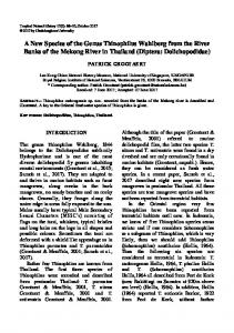
calls. Consider the memory configuration for the 4-element list of fig. 3(a) at the fourth invocation of the rev() function. This memory configuration is shown in fig. 4(a), where the ARS has been included to maintain the pointer links for x in previous calls of rev(), and the explicit representation of the L, PL, SL, and CLS sets have been omitted for simplicity. The information within the ARS is required when we return to an enclosing call, so that we know the destinations of local pointers.

(a)

rev pl1= rev pl1= rev pl1= rev pl1= main pl1= ARS

pl1

l1

l2

sl1

l3

sl2

pl1= sl1= sl2= sl3= sl4=

rfsl1

rfsl2

rfsl3

l1 PC={x}

(b)

rfpl1

l2

rfpl1= rfsl1= rfsl2= rfsl3= rfsl4=

pl1= sl1= sl2= sl3= sl4=

x

*

PC={x}

sl2

*

rfsl1 n1 PC={x}

(c)

sl1 pl1= sl1= sl2= sl3= sl4=

* PC={x}

rfpl1= rfsl1= rfsl2= rfsl3= rfsl4=

l4

|

sl4

x

n2

sl2

mc4St9

CLS(l1)= CLS(l2)= CLS(l3)= CLS(l4)=

rfpl1

rfsl3

|

rfsl4 pl1

sl3

x rfptr rfsl2

sl4

CLS(l1)= CLS(l2)= CLS(l3)= CLS(l4)=

l3

PC={x}

sl1

l4

sl3

x rfptr

*

mc4St9

x

sl3

sg4St9

rfsl4 pl1

n3

sl4

|

CLS1(n1)= CLS2(n1)= CLS1(n2)= CLS1(n3)=

Figure 4: The role of recursive flow links in interprocedural analysis: (a) memory configuration with its ARS; (b) the same memory configuration from (a) described with recursive flow links; (c) the shape graph that abstracts the memory configuration in (b). Somehow we need to translate the information provided by the ARS into the abstract domain, so that we can analyze recursive programs. The key elements to provide that information are recursive flow links, which allow us to recover the state of pointers when returning to enclosing recursive calls through a simple pointer tracing mechanism.

4.1

Recursive flow links

We define the recursive flow pointer link and recursive flow selector link, very similarly to regular pointer links and selector links. However, these links do not represent actual links existing in the program data structure but 7

rather trace the positioning of pointers along the recursive, interprocedural control flow. For these new links, we need to define a set of recursive flow pointers (RFPTR) and a set of recursive flow selectors (RFSEL), so the set of recursive flow pointer links (RFPL) and the set of recursive flow selector links (RFSL) can be built upon them. By convention, recursive flow pointers are named after the pointer variables that they trace, with the subscript rf ptr. They point to the same memory location/node where the original pointer was pointing to in the previous call in a stack of recursive calls. Recursive flow selectors are also named after the pointer that they trace, but with the subscript rf sel. They are used to trace pointers back in the sequence of calls beyond the immediately previous activation record. The traced pointer, along with its recursive flow pointer and recursive flow selectors are referred to as the ptr-rfptr-rfsel trio. TLTf un holds the set of all these Tracing Links Trios for function f un. Fig. 4(b) shows the memory configuration from (a), exchanging the ARS for the needed recursive flow links, which are shown in dashed lines. Here, the ptr-rfptr-rfsel trio x-xrf ptr -xrf sel is considered. A new location/node, denoted by * has been added to mean ”no location”, acting like a NULL for the recursive flow path. Following the trace through a recursive flow selector link with * as destination would not correspond to any activation record in the succession of recursive calls, and therefore would not render any realistic memory configuration. For interprocedural analysis, the definitions for memory configurations and shape graphs are updated as follows: mcSti ∈ MCSti , mcSti = ; sgSti ∈ SGSti , sgSti = . Coexistent links sets are now expanded to accommodate the new link types. In the concrete domain CLS(l) ∈ CLS, l ∈ L, CLS(l) = . For example, in the fig. 4(b) consider CLS(l3), which has PL(l3)={∅}, SL(l3)i={sl2}, SL(l3)o={sl3}, RFPL(l3)={rfpl1}, RFSL(l3)i={∅} and RFSL(l3)o={rfsl3}. In the abstract domain, CLSj(n) ∈ CLS, n ∈ N, CLSj(n) = . Note that nodes that are or have been pointed by a recursive flow pointer are marked with a special property, the previous call (P C) property, which indicates the set of pointers that have pointed to the node in the course of the traversal implicit in the sequence of recursive calls. In the abstract domain, this property will prevent the summarization of nodes that have been visited during the analysis with nodes that have not yet been visited. Fig. 4(c) shows the abstraction of the memory configuration in (b). Here memory locations l1 and l2 are summarized by just n1. The selector links are updated accordingly as shown in the figure. Here we can understand the role played by coexistent links sets: they discriminate what links can be combined to form real memory configurations out of n1. For example, we know that rfsl1 and sl2 cannot exist together over a memory configuration represented by n1.

4.2

Context change rules

We have stated that shape graphs are transformed while flowing in and out of functions, so that they are suitable for the new context. This is done with the call-to-start (CTS) rule, and the return-to-call (RTC) rule. For these rules we need to introduce the concept of apptr-fpptr pair, which is a pair of pointers related by a actual parameter vs formal parameter relationship for a given function call. For instance, l-x is an apptr-fpptr pair for the call at statement 22 in fig. 1, and z-x forms an apptr-fpptr pair for the call at statement 13. AFPf un is the set of all apptr-fpptr pairs for function f un. The algorithms presented in this section also make use of a few functions that are worth mentioning (fig. 5). For example, the set pl(ptr,n,sg) function is responsible for updating the pointer link defined for pointer ptr so that it gets to point to node n in shape graph sg. This may involve a destructive updating, if ptr was already pointing to some other node. The set rfpl(rfptr,n,sg) function works in the same way but with recursive flow pointer rfptr (with set [rf]pl() we refer to set pl() or set rfpl()). The set rfsl(n1,rfsel,n2,sg) function updates recursive flow selector rfsel so that it starts at n1 and ends at n2, all within sg. Again, this may involve breaking a connection existing previously. The remove pl(ptr,sg), remove rfpl(rfptr,sg) and remove rfsl(rfsel,sg) are in charge of removing unneeded pointer links, recursive flow pointer links and recursive flow selector links, respectively, when they are no longer needed after the context change. All these operations update the [RF]PL (i.e., PL or RFPL), [RF]SL (i.e., SL or RFSL), and CLS sets in the shape graph accordingly. For example, when adding a new pointer link to a shape graph with set pl(ptr,n,sg), this involves adding it to the PL set (statement 5, algorithm set [rf]pl(), fig. 5), as well as adding it to every CLSj(n) ∈ CLS (statement 6, algorithm set [rf]pl(), fig. 5). Also, the operations just mentioned are responsible for performing all the graph normalization operations (by summarizing compatible nodes) that may be required. Another aspect that should be considered for the CTS and RTC rules is that program must be preprocessed so that formal parameters are not modified inside the procedure. These restrictions make the formulation simpler and do not involve any loss of generality, as it is always possible to rewrite a function to comply with these 8

1: 2: 3: 4: 5: 6: 7: 8:

1: 2: 3: 4: 5: 6: 7: 8: 9: 10: 11: 12: 13:

1: 2: 3: 4: 5: 6:

1: 2: 3: 4: 5: 6: 7: 8:

Algorithm set [rf]pl([rf]ptr,n,sg) Input: [Recursive flow] pointer to be set, [rf]ptr Node where the pointer [rf]ptr must point to, n Input shape graph, sg = Output: Resulting graph, sg begin algorithm if ( ∃ [rf]pl ∈ [RF]PL / [rf]pl=, n2 ∈ N ) then ∀ CLSj(n2) ∈ CLS, remove [rf]pl from CLS Remove [rf]pl from [RF]PL end if Add [rf]pl= to [RF]PL ∀ CLSj(n) ∈ CLS, add [rf]pl to CLSj(n) Normalize graph by summarizing compatible nodes return sg end algorithm Algorithm set rfsl(n1,rfsel,n2,sg) Input: Node where the recursive flow selector link must originate, n1 Recursive flow selector used for the recursive flow link, rfsel Node where the recursive flow selector link must terminate, n2 Input shape graph, sg = Output: Resulting graph, sg begin algorithm foreach ( n3 ∈ N / ∃ rfsl= ∈ RFSL) ∀ CLSj(n3), remove rfsl from CLSj(n3) ∀ CLSj(n1), remove rfsl from CLSj(n1) Remove rfsl from RFSL end foreach Add rfsl= to RFSL if ( n1 != n2 ) then ∀ CLSj(n1) ∈ CLS, add rfsl as outgoing to CLSj(n1) ∀ CLSj(n2) ∈ CLS, add rfsl as incoming to CLSj(n2) else /* n1 == n2 */ ∀ CLSj(n1) ∈ CLS, add rfsl as cyclic to CLSj(n1) end if return sg end algorithm Algorithm remove [rf]pl([rf]ptr,sg) Input: [Recursive flow] pointer whose [recursive flow] pointer links must be removed from the graph, [rf]ptr Input shape graph, sg = Output: Resulting graph, sg begin algorithm if ( ∃ [rf]pl ∈ [RF]PL / [rf]pl= ∈ [RF]PL, n ∈ N ) then Remove [rf]pl from [RF]PL ∀ CLSj(n) ∈ CLs, remove [rf]pl from CLSj(n) end if Normalize graph by summarizing compatible nodes return sg end algorithm Algorithm remove rfsl(rfsel,sg) Input: Recursive flow selector whose recursive flow selector links must be removed, rfsel Input shape graph, sg = Output: Resulting graph, sg begin algorithm foreach ( n1 ∈ N ) foreach ( n2 ∈ N / ∃ rfsl= ∈ RFSL ) ∀ CLSj(n1) ∈ CLS, remove rfsl from CLSj(n1) ∀ CLSj(n2) ∈ CLS, remove rfsl from CLSj(n2) Remove rfsl from RFSL end foreach end foreach return sg end algorithm

Figure 5: Base functions for use in the context change rules.

9

conditions by using additional variables, whenever parameters are passed by value. When parameters are passed by reference, they are treated just like global pointers. The call-to-start rule determines how the heap is transformed from a function call site to the context inside the function called. Fig.6 shows the algorithm for the CTS rules, both recursive (CTSrec ) and non-recursive (CTSnrec ) versions. Mainly, these rules involve assigning pointer formal parameters to where actual parameters are pointing to, by processing all available apptr-fpptr pairs for the function. This is done in step 1 in CTSnrec and step 3 in CTSrec (fig. 6). CTSnrec also performs some initialization of the shape graph for the new context, while CTSrec is also responsible for updating recursive flow links so we can recover the previous context later. Algorithm CTSnrec (sg,PTR,GLB,PTRf un ,RFSELf un ,AFPf un ) Input: Input shape graph, sg = Set of all pointers in the program, PTR Set of global pointers, GLB Set of locally defined pointers plus pointer formal parameters in the function, PTRf un Set of recursive flow selectors for the function, RFSELf un Set of apptr-fpptr pairs for the function, AFPf un Output: Resulting graph after the context change, sg begin algorithm STEP 1: /* Assign formal parameters based on actual parameters */ 1: foreach apptr-fpptr pair ∈ AFPf un 2: Get pl ∈ PL / pl = 3: Run set pl(fpptr,n,sg) 4: if (apptr ∈ / GLB) then 5: Run remove pl(apptr,sg) 6: end if 7: end foreach STEP 2: /* Initialize shape graph for new context */ 8: ∀ ptr ∈ PTR / ptr ∈ / PTRf un and ptr ∈ / GLB, run remove pl(ptr,sg) 9: ∀ rfsel ∈ RFSELf un and ∀ n ∈ N, run set rfsl(n,rfsel,*,sg) 10: return sg end algorithm

1: 2: 3: 4: 5: 6: 7: 8: 9: 10: 11: 12: 13: 14: 15: 16: 17: 18: 19: 20: 21: 22: 23: 24: 25:

Algorithm CTSrec (sg,PTRf un ,RFPTRf un ,AFPf un ,TLTf un ) Input: Input shape graph, sg = Set of locally defined pointers plus pointer formal parameters in the function, PTRf un Set of recursive flow pointers for the function, RFPTRf un Set of apptr-fpptr pairs for the function, AFPf un Set of tracing links trios ptr-rfptr-rfsel for the function, TLTf un Output: The resulting graph after the context change, sg begin algorithm STEP 1: /* Clean up shape graph for new context */ foreach ptr ∈ ( PTRf un ∪ RFPTRf un ) Get pl ∈ (PL ∪ RFPL) / pl = Add pl to RefPL, where RefPL is an auxiliary pointer link set Run remove pl(ptr,n,sg) end foreach STEP 2: /* Assign recursive flow pointers and recursive flow selectors as needed */ foreach ptr-rfptr-rfsel trio ∈ TLTf un Get pl ∈ RefPL / pl = Get rfpl ∈ RefPL / rfpl = if (n1 == NULL and n2 == NULL) then /* Do nothing, ptr is yet to be assigned */ else if (n1 != NULL and n2 == NULL) then Run set rfpl(rfptr,n1,sg) Add rfptr to PC property for n1 else if (n1 != NULL and n2 != NULL) then Run set rfpl(rfptr,n1,sg) Add rfptr to PC property for n1 Run set rfsl(n1,rfsel,n2,sg) else /* n1 == NULL and n2 != NULL*/ Abort analysis. Case not supported. end if end foreach STEP 3: /* Assign formal parameters based on actual parameters */ foreach apptr-fpptr ∈ AFPf un Get pl ∈ RefPL / pl = Run set pl(fpptr,n,sg) end foreach return sg end algorithm

Figure 6: The call-to-start rules, to change the heap context when entering a function. 10

The tracing of pointers in a sequence of recursive calls through recursive flow links and context change rules has a limitation though, as may be guessed from statement 18 in fig. 6. If for a ptr-rfptr-rfsel trio ∈ TLTf un , we find that rfptr is pointing to some non-NULL node but ptr is not assigned, we cannot continue the recursive trace of that pointer and the analysis can no longer continue. This case is found when there is more than one recursive call to the same function and is possible to have a gap of 2 or more recursive calls before assigning a local pointer. Fortunately and according to our experience, these cases can be rewritten to an equivalent version that avoids the gap in the recursive flow path, just by reordering a few statements in a way that preserves the program behavior, like in fig. 7. In the context of current compilers, this transformation is very simple and can be performed by a previous step in the compilation process.

Figure 7: Two versions of a program that creates a binary tree: (a) produces a gap in the recursive flow path so it cannot be analyzed by our technique; (b) prevents that gap with a simple statement reordering and makes the program analyzable while preserving its meaning.

1: 2: 3: 4: 5: 6: 7: 8: 9: 10: 11: 12: 13: 14: 15: 16: 17: 18: 19: 20:

Algorithm RTCnrec (sg,cs,return ptrf un ,PTRf un ,RFPTRf un ,RFSELf un ,GLB,AFPf un ) Input: Input shape graph, sg = Call site where we return to, cs = Pointer returned by the function return statement, return ptrf un Set of locally defined pointers plus pointer formal parameters in the function, PTRf un Set of recursive flow pointers for the function, RFPTRf un Set of recursive flow selectors for the function, RFSELf un Set of global pointers, GLB Set of apptr-fpptr pairs for the function, AFPf un Output: Resulting graph after the context change, sg begin algorithm STEP 1: /* Assign pointer at call site */ Get pl = ∈ PL Run set pl(assigned ptr,n,sg) Run remove pl(return ptrf un ,sg) STEP 2: /* Assign actual parameters based on formal parameters */ foreach apptr-fpptr pair ∈ AFPf un Get pl = ∈ PL if (apptr ∈ GLB) then Get pl2 = ∈ PL if (n1 != n2) then return empty graph, as it does not represent a realistic memory configuration. end if else Run set ptr(apptr,n1,sg) end if Run remove pl(fpptr,sg) end foreach STEP 3: /* Clean up shape graph for new context */ ∀ ptr ∈ PTRf un , run remove pl(ptr,sg) ∀ rfptr ∈ RFPTRf un , run remove rfpl(rfptr,sg) ∀ rfptr ∈ RFPTRf un and ∀ n ∈ N, remove rfptr from PC property for n ∀ rfsel ∈ RFSELf un , run remove rfsl(rfsel,sg) return sg end algorithm

Figure 8: The non-recursive version of the return-to-call rule. 11

1: 2: 3: 4: 5: 6: 7: 8: 9: 10: 11: 12: 13: 14: 15: 16: 17: 18: 19: 20: 21: 22: 23: 24: 25: 26: 27:

Algorithm RTCrec (sg,rcs,return ptrf un ,PTRf un ,AFPf un ,TLTf un ) Input: Input shape graph, sg = Recursive call site where we return to, rcs = Pointer returned by the function return statement, return ptrf un Set of locally defined pointers plus pointer formal parameters in the function, PTRf un Set of apptr-fpptr pairs for the function, AFPf un Set of tracing links trios ptr-rfptr-rfsel for the function, TLTf un Output: The set of graphs resulting from the context change, SGout begin algorithm STEP 1: /* Assign pointer at call site */ if (return ptrf un != assigned ptr) then Get pl = ∈ PL Run set pl(assigned ptr,n,sg) end if Add assigned ptr to updatedPTR, where updatedPTR is an auxiliary pointer set STEP 2: /* Assign actual parameters based on formal parameters */ foreach apptr-fpptr pair ∈ AFPf un Get pl = ∈ PL Add pl to formalPL, where formalPL is an auxiliary pointer link set end foreach foreach pl = ∈ formalPL Run set pl(apptr,n,sg) Add apptr to updatedPTR end foreach STEP 3: /* Update remaining pointers and recursive flow links, if needed */ nonupdatedPTR = PTRf un - updatedPTR, where nonupdatedPTR is an auxiliary pointer set foreach ptr-rfptr-rfsel trio ∈ TLTf un if (ptr ∈ nonupdatedPTR) then Get rfpl = ∈ RFPL Run set ptr(ptr,n,sg) Add ptr to updatedPTR Remove rfptr from PC property for n Store in SGout graphs resulting from updating rfptr through rfsel ∀ sgout ∈ SGout , run set rfsl(n,rfsel,*,sg) end if end foreach nondefinedPTR = PTRf un - updatedPTR, where nondefinedPTR is an auxiliary pointer set ∀ ptr ∈ nondefinedPTR and ∀ sgout ∈ SGout , run remove pl(ptr,n,sgout ) return SGout end algorithm

Figure 9: The recursive version of the return-to-call rule. The CTS rule is therefore used to transform the heap context when entering to a function. On the other hand, the return-to-call (RTC) rule transforms the heap returned by a function to the calling site. Fig. 8 describes the algorithm for RTCnrec , while fig. 9 does the same for RTCrec . To explain these RTC rules, we first need to differentiate the pointer returned by a function f un, called return ptrf un , from the pointer assigned at the call site where we return to, called assigned ptr. For example, return ptrf un = y for the rev() function (statement 18, fig. 1) and assigned ptr = r when returning to the main() function (statement 22 , fig. 1). Then we introduce the call site (cs), as a tuple that contains the required information of a given call site. It is described as cs = , where assigned ptr is the pointer assigned at the call site where we return to, as we have just described, and actualPTR is the set of pointer actual parameters involved in the call. For example, actualPTR = {l} for the call site at statement 22 in the reverse program (fig. 1). However, for recursive call sites, such as statement 13 in reverse (fig. 1), we need another piece of information, the backward propagation path (bpp) associated to the recursive call site (for example, bpp1 in fig. 2). Therefore a recursive call site is a tuple rcs = . The backward propagation paths within recursive call sites are used by the shape graph propagation algorithm, which is described in section 4.3. As step 1, the RTC rules assign the pointer returned by the function return ptrf un , if any, to the pointer assigned at the calling site, assigned ptr. For example, upon returning to statement 22 in fig. 1, r (assigned ptr) is made to point to where y (return ptrf un ) is pointing to. Then, actual parameters from the enclosing call must be made to point to the nodes pointed to by formal parameters in the returning function (step 2 in RTCnrec and RTCrec ). Finally, in step 3, RTCnrec must clean up unneeded elements for the new context, while RTCrec must update local pointers not already updated in step 2, by using available recursive flow links, and then update them as well to reflect the change of context. Note that RTCrec returns a set of graphs for every input. This is caused by statement 21 in fig. 9, which may produce shape graphs with different pointer aliasing arrangement, which causes the analysis to represent them in separate graphs. This is the case when there are 2 possibilities by tracing back 12

a recursive flow selector, typically another node (there are more enclosing recursive calls) or * (last recursive call in the ARS). 4.2.1

Example x

x rfptr *

sl3

n1

x rfptr *

n1

PC={x}

*

n2

sg2St12

z

x *

n3

*

n4

n1

PC={x}

n2

*

PC={x}

n3

n3

*

n4

sl2

|

CLS1(n3)=

{sg3 St13} = RTCrec (sg2 St18 ,rcs,y,{x,y,z},{z−x},{x−xrfptr −xrfsel}) rcs =

x rfptr

*

sl1

sg2St18

z

sg3St9

x

x rfptr

PC={x}

pl1= sl1= sl2= sl3=

|

sg3 St9 = CTS rec (sg2 St12 ,{x,y,z},{x rfptr},{x−z},{x−xrfptr −xrfsel})

*

n2

PC={x}

y

pl1

*

n4

*

|

n1

PC={x}

(a)

x *

n2

y

z *

n3

*

n4

sg3St13 |

(b)

Figure 10: Examples of the effect of (a) the CTSrec rule and (b) the RTCrec rule. Context change rules are better understood by means of a example. Fig. 10(a) shows how the CTSrec rule acts upon shape graph sg2St12 , the abstraction of 4-element singly-linked list at the third call to rev(). Statement 12 is just a special kind of statement that filters out any possible graphs that do not verify the condition z != NULL, and thus have no sense in the if branch. The result of applying the CTSrec rule is named sg3St9 . Null assigned or uninitialized pointers are not shown. Links are only displayed graphically, and coexistent links sets are left out, to simplify the presentation. Note that the location pointed to by z in sg2St12 is now pointed to by x in sg3St9 . This has been done in step 3 for the CTSrec rule (fig. 6) by using the apptr-fpptr pair z-x. The xrf ptr pointer is updated to point to n2, node pointed to by x in the previous context, and the recursive flow selector from n2 to n1 in sg3St9 leaves the trace to the node pointed to by xrf ptr in the previous context. This is the effect of step 2 for CTSrec . Fig. 10(b) shows how the RTCrec rule acts upon the shape graph returning from the third rev() call, labeled as sg2St18 . The result is sg3St13 , which exchanges actual parameter z for its paired formal parameter x (step 2 in the RTCrec rule, fig. 9), which in turn is updated to the location marked by xrf ptr in sg2St18 (step 3 in the same rule). The recursive call selector link emanating from n2 in sg2St18 serves to update the recursive flow pointer xrf ptr to point to n1 in sg3St13 . Note that step 1 for the RTCrec rule has no effect in this case as the pointer returned by the function, y, is the same pointer assigned at the call site. An interesting fact about the use of coexistent links sets in our abstraction can also be observed in fig. 10(b). Coexistent links sets for node n3 are shown for sg2St18 . They reflect that n3 is now pointed to by 2 different nodes through the selector nxt. This is highlighted graphically by shading the oval depicting the node. This accuracy about knowing not only that the node is shared, (i.e., it can be reached from at least 2 other nodes), but also knowing how it is shared, is made possible by the coexistent links sets and is a unique feature of our shape analysis strategy. Furthermore, this sharing pattern can be undone as will occur in the following execution of statement 14. Thus, we will be able to preserve the listness property of the structure at the end of the function. A final consideration about the use of recursive flow links: we have seen that we can recover the destination of pointers in previous recursive calls either by (i) matching formal and actual parameters, (ii) assigning returned pointers or (iii) through recursive flow links (rfptrs and rfsels). In fact, we could add a ptr-rfptr-rfsel trio for every pointer ptr ∈ PTRf un , i.e., for every pointer which is locally defined or a formal parameter. This would work out fine. However, this is not needed in most cases and complicates the shape graphs unnecessarily, as some 13

pointers do not need to trace back its position through recursive flow links. Only pointers which are live (used before defined) after a recursive call and cannot be recovered by (i) or (ii) need a ptr-rfptr-rfsel trio. To control this, we have added a special statement that determines what pointers do not need such a trio. A compiler pass running prior to the shape analyzer takes care of this decision through live pointer analysis. Statement #pragma SAP.no rflinks for(y,z) in the reverse example indicates that we do not need recursive flow links for y (returned value) and z (matched with formal parameter x). This statement is only considered by the preprocessing module as a start-up setting for the analysis and does not induce any other changes along the analysis.

4.3

Shape graph propagation

The flow of the analysis is determined by the cycles of forward and backward propagation, which are controlled by the graph propagation algorithm. Inherent to the idea of graph propagation is the concept of propagation paths, which are hierarchical sub-trees of statements that determine a control flow path within a recursive function. A forward propagation path, fpp, is a subtree of statements corresponding to a control flow path starting at the function entry and ending either at the return statement or at a recursive call. A backward propagation path, bpp, is very similar, only that it starts at a recursive call site. FPPf un is the set of forward propagation paths available for function f un. BPPf un is therefore the set of backward propagation paths for f un. A recursive call site, defined previously as rcs = , includes bpp, the backward propagation path for the recursive call site rcs ∈ RCSf un , where RCSf un is the set of all recursive call sites for function f un. For the reverse example, the sequence of statements 10, 11, 12, 13 forms fpp1 ∈ FPPrev and the sequence 10, 11, 16, 17, 18 forms fpp2 ∈ FPPrev . On the other hand, the sequence 14, 15, 18 forms bpp1 ∈ BPPrev . These propagation paths are drawn in fig. 2. A propagation cycle consist in the analysis of an entry shape graph through all available propagation paths. A forward propagation cycle starts with a graph reaching the function entry, while a backward propagation cycle starts with a graph returning to a call site. Starting graphs for propagation cycles must have been previously transformed by applying the appropriate context change rule. From a practical point of view, it should be noted that common statements in propagation paths (like 10 and 11 for fpp1 and fpp2) are only analyzed once per input shape graph. The graph propagation algorithm is described in fig. 11. It needs, among other input parameters, all the available information for the analyzed function, which is contained in FDATAf un = . PTRf un is the set of locally defined pointers for the function (including formal parameters). RFPTRf un and RFSELf un are the sets of recursive flow pointers and recursive flow selectors defined for the function. return ptr is the pointer variable returned by the function return statement. AFPf un is the set of Actual parameter vs Formal parameter Pairs; TLTf un is the set of Tracing Links Trios; FPPf un is the set of Forward Propagation Paths; finally, RCSf un is the set of Recursive Call Sites. All the information in FDATAf un is gathered by the preprocessing pass and available at the start of the analysis. The process of graph propagation is invoked whenever a call to an external function (i.e., not a recursive call) is encountered in the analysis. In fact, the analysis starts by invoking the graph propagation algorithm over a call to the main() function. The process described in fig. 11 is repeated for every input graph reaching the function call. As a first step, the input graph is put into context by the CTSnrec rule. The resulting graph is added to the FPSG set, which contains all Forward Propagated Shape Graphs. While this set is not empty the analysis will continue to propagate the available shape graphs through the different forward propagation paths in the function body. Shape graphs will be modified according to the abstract semantics of the statements along those paths. Some of the forward propagation paths will encounter a recursive call, like fpp1 in the reverse example (fig. 2, through the if branch). Graphs following such paths can be used for another cycle of forward propagation, by first calling CTSrec and then adding the result to FPSG. However, the resulting graph from the CTSrec rule is only added to FPSG if it contains information that has not already been analyzed, for example a new node with a new link. There will surely be one forward propagation path that reaches the return statement, like fpp2 in the reverse example (fig. 2, through the else branch). Shape graphs following this path will be added to the SGret set, which will accumulate configurations reaching the end of the function during the analysis. Besides, all graphs reaching the return statement (remember that the function must have been previously normalized to contain only one return statement as the last statement in its body), are suitable to feed the backward propagation cycle. Before that, the graphs must be put into the appropriate context by the RTCrec rule. Graphs achieved this way are added to the BPSGrcs set, which contains the Backward Propagated Shape Graphs for the recursive call site rcs. 14

1: 2: 3: 4: 5: 6: 7: 8: 9: 10: 11: 12: 13: 14: 15: 16: 17: 18: 19: 20: 21: 22: 23: 24: 25: 26: 27: 28: 29: 30: 31: 32: 33: 34: 35: 36: 37: 38: 39: 40: 41: 42: 43: 44: 45:

Algorithm graph propagation(sg,PTR,GLB,cs,FDATAf un ) Input: Input shape graph, sg = Set of local pointers for the function, PTRf un Set of global pointers, GLB Call site that calls the function, cs All available data for the function, FDATAf un = Output: Set of graphs that describe the behavior of the function for input sg, SGout begin algorithm Run sg = CTSnrec (sg,PTR,GLB,PTRf un ,RFSELf un ,AFPf un ) Add sg to FPSG, set of shape graphs for forward propagation while (FPSG 6= ∅) Extract sg from FPSG foreach (fpp ∈ FPPf un ) Transform sg according to abstract semantics of fpp if (last statement in fpp is the return statement) then Add sg to SGret foreach rcs ∈ RCSf un Run sg = RTCrec (sg,rcs,return ptrf un ,PTRf un ,AFPf un ,TLTf un ) if (sg contains info not already analyzed at rcs) then Add sg to BPSGrcs , set of shape graphs for backward propagation at recursive call site rcs end if end foreach else /* last statement in fpp is a recursive call */ Run sg = CTSrec (sg,PTRf un ,RFPTRf un ,AFPf un ,TLTf un ) if (sg contains info not already analyzed at function entry) then Add sg to FPSG end if end if end foreach while (some BPSGrcs 6= ∅, rcs = ∈ RCSf un ) Extract sg from BPSGrcs Transform sg according to abstract semantics of bpp if (last statement in bpp is the return statement) then Add sg to SGret foreach rcs2 ∈ RCSf un Run sg = RTCrec (sg,rcs2,return ptrf un ,PTRf un ,AFPf un ,TLTf un ) if (sg contains info not already analyzed at rcs2) then Add sg to BPSGrcs2 end if end foreach else /* last statement in bpp is a recursive call */ Run sg = CTSrec (sg,PTRf un ,RFPTRf un ,AFPf un ,TLTf un ) if (sg contains info not already analyzed at function entry) then Add sg to FPSG end if end if end while end while foreach (sg ∈ SGret ) Run sg = RTCnrec (sg,cs,return ptrf un ,PTRf un ,RFPTRf un ,RFSELf un ,GLB,AFPf un ) Add sg to SGout end foreach return SGout end algorithm

Figure 11: The graph propagation algorithm, which controls the cycles of forward and backward propagation.

The backward propagation cycle works in a similar fashion to the forward propagation cycle. Paths that encounter a recursive call may enlarge the FPSG set. Paths that reach the return statement enlarge SGret , and at the same time, are seeded as new shape graphs for backward propagation cycles, provided that they contain information that has not been already analyzed. The cycles of forward and backward propagation terminate when the FPSG set and all BPSGrcs sets are empty, and thus all possible configurations have been captured. The last step before returning to the call site that triggered the propagation process is transforming the shape graphs accumulated for the return statement, SGret , to the context of the calling site. This is done by applying the RTCnrec rule. The output achieved is a set of graphs, SGout , that captures all possible configurations that the function may produce from the input shape graph. 15

5

Optimization by reusing previous analysis

The technique described so far is able to provide correct shape graph abstractions for generic interprocedural programs, albeit maybe requiring some statement rearrangement as hinted in section 4.2. However, it can be enhanced by reusing computed effects for functions in the case of similar inputs. This saves the effort of reanalyzing a function unnecessarily and is done by tabulating input and output graphs for the function. On entry to a function, the input shape graph is split based on reachability information derived from so-called reaching pointers. These are the pointers passed as parameters to the function as well as the global pointers used in the function, i.e., the pointers that can be used within the function to access the structure. First, all nodes and links that may be in a traversal through the structure starting on the reaching pointers are registered. Then the registered elements are used to create a new graph, the reachable graph, which is the part of the shape graph which corresponds to the part of the heap which is accessible within the function. Conversely, the unreachable graph corresponds to the part of the heap which is inaccessible within the function and it is determined by following possible pointer-chasing paths starting with the non-reaching pointers, i.e., the rest of pointers in the program which are live at the point of the call. Fig. 12 outlines our mechanism to reuse previous analysis based on tabulation of input-output pairs and splitting by reachability. The input shape graph, sgin , is split into the reachable graph, sgreach , and the unreachable graph, sgureach , based on the reaching and non-reaching pointers for the function. If the graph resulting from the context change enforced by CTSnrec , sgCT S , has already been analyzed, then we can use the output previously tabulated, and thus save its analysis with the graph propagation algorithm. Whatever the case, the shape graphs that model the behavior of the function for input sgCT S are gathered in SGret . Then, the graphs resulting from the context change performed by RTCnrec , SGRT C , are joined with the unreachable graph, sgureach , which was obtained at the function entry. Finally, SGout will contain the final output, which captures the complete effect of the function over the input shape graph. Consider a variant of the reverse example in fig. 1, where instead of creating one list reached through pointer l, we create two lists reached through pointers l1 and l2 respectively, where l1 and l2 are locally defined for main(). Now consider a call to the rev() function over l1 (r1 = rev(l1)). The input graph to the function, sgin , is that of the 2 lists reached through l1 and l2. The graphs for this example are embedded in fig. 12, where the lists are considered longer than 3 elements for simplicity. Note that the 2 lists do not share elements even though it could seem so, by looking at the graph for sgin . A thorough look at the coexistent links sets for this graph reveals that the lists are independent. Splitting by reachability in such scenario would yield the list reached through l1 as the reachable graph, sgreach , and the list reached by l2 as the unreachable graph, sgureach . Shape graphs in fig. 12 continue to show possible graphs resulting from the analysis: sgCT S as the graph to be compared against the tabulated input graphs for the function; sgret as the result from the analysis; sgRT C as the result put back into the context of the calling site; and finally sgRT C is joined with sgureach , to produce sgout , which captures the overall effect of the function call. The combination of a graph splitting mechanism with input-output tabulation, allows to reuse function analysis for the whole range of different input graphs whose reachable part of the graph, after the context change, has been previously analyzed. For example, in the variant proposed in this section, after calling to rev() over l1, a subsequent call over l2 (r2 = rev(l2)) would reuse the effect determined for rev() in the first call, because the shape graph entering the context of the rev() function,sgCT S , is again a single list reached through formal parameter x. It should be noted though, that not every input graph can be split. If there is any coexistent links sets for any node indicating that it can be reached both from a reaching pointer and non-reaching pointer, then the heap cannot be split. Otherwise, it could not be reconstructed upon exit just by a simple join operation. In that case, the whole graph is analyzed. This limitation is similar to the concept of cutpoint defined in [13], only slightly more restrictive. However, when unable to split the graph by reachability, [13] must abandon the analysis, while we can carry on, albeit with the whole representation of the heap. Despite this limitation, the optimization described here allows to reuse the analysis of many functions that create and/or manipulate dynamic data structures. As a glimpse into the benefits of this optimization, we conducted a small test. First, we run the interprocedural analysis of the reverse example, which took 0.22 seconds in a Pentium4 3GHz. Then we introduced a variation in the example to reverse the list 8 times, by calling the rev() function 8 times in total. The analysis took 0.66 seconds in that case. Then, we enabled the optimization described in this section, and the analysis reduced its time to 0.27 seconds, by being able to reuse the effect of the first call to rev() for the subsequent 7 calls. 16

Figure 12: Flow chart of graph splitting by reachability and input-output shape graph tabulation to reuse computed function effects.

6

Related work in interprocedural shape analysis

Next we present the most relevant works to our aim of achieving interprocedural support for shape analysis. Hackett and Rugina [4] present a novel shape analysis abstraction built on top of a region points-to analysis, which is suitable for interprocedural support. Their analysis is based on local reasoning over individual heap locations, called tracked locations. By avoiding to analyze the heap as a whole, they can achieve a fast analysis (less than a minute for tens of thousands of C code for a bug detection extension). However, their analysis relies heavily on the underlying points-to analysis. If it cannot determine enough disjoint regions, the analysis will not be accurate enough. Marron et. al [10] describe a shape analysis algorithm that sort of combines ideas from [15] and [3], to achieve shape graphs where nodes can represent a predefined topology. Their analysis is fast, mainly due to the simplification achieved in the operations over the normalized form of the graphs. They seem to be able to analyze programs more complex than other related work although the ideas for recursive function support, which the authors describe as ”crude”, are not described. There is another body of work built as extension to the 3-valued logic analyzer (TVLA) as described in [9]. These works ([8], [12], [13]) are sound and illustrating. We regard them as the reference works in shape analysis. 17

However, all works derived from the TVLA system need that the programmer designs some specific predicates that encode the characteristics of memory that are needed for a correct analysis. This is no trivial task and requires thorough knowledge of the system, so we think these works are not tailored for parallelizing compilers. In our approach, on the contrary, the programmer does not need any specific knowledge about the shape analysis technique. Jeannet et. al [8] rely on the computation of summary transformers for functions, by data flow equation solving with modified operators. This is done by using a double vocabulary of predicates to encode the relationship between input and output states. However, the analysis in this work proves to be very costly to the point that it is unable to complete for some simple programs that manipulate binary trees, due to combinatorial explosion of possibilities in the analysis. Rinetzky and Sagiv [12] explore the idea of abstracting the activation record stack as a new entity in the graphs to track the locations of pointers in a sequence of recursive calls. This simple idea and a few new predicates yield an interesting interprocedural shape analysis technique, whose use is only reported for singly-linked lists and suffers from scalability problems, due to the impossibility to recognize the relevant context for a function analysis and the need to reanalyze a function for every call, even in the case of the same input heap. Rinetzky et. al [13] improve their previous efforts with an extension that is able to reuse computed function summaries very efficiently by using a tabulation algorithm that relies on context change rules upon entering to and exiting from functions, and some specific predicates. However, some heap sharing patterns between pointers cannot be solved by their context change rules and therefore, programs that contain any such pattern cannot be analyzed.

7

Experimental results

We have implemented the algorithms presented in this paper (including the optimization described in section 5) to extend our previous shape analyzer framework [16]. In this section we present some results from early experiments. Our first aim was twofold: (i) to prove that the algorithm works and yields correct results for a variety of programs that manipulate dynamic data structures, and (ii) to measure its performance in terms of analysis time and required memory compared to [13], which describes what we think is the most complete interprocedural shape analysis to date. Therefore, we have focused initially on a subset of the codes tested in [13], so we can establish a common ground for comparison. These are simple yet meaningful interprocedural programs that feature recursive algorithms. They deal with singly-linked lists or binary trees. Both [13] and our method are able to determine that the invariants of the structure are preserved after the call to the recursive functions. This means that for the list tests, if the function is called with an acyclic singly-linked list, then the output is also an acyclic singly-linked list, i.e., no cycles have been introduced in the list and no memory leaks have occurred, so the listness property is preserved. For the tree tests, if the input is an unshared binary tree (no child has 2 parents), we check that the shape is preserved at the output. [13] also analyzes some sorting programs over singly-linked list to verify sortedness in lists. We do not focus on verification, but rather on memory description toward dependence analysis in the context of parallelizing compilers, so we do not consider these tests. Table 1 presents the comparison in analysis time and memory consumed between the results presented in [13] and our own results. The testing platform for [13] is a Pentium M 1.5 GHz with 1 GB. Our platform is a Pentium M 1.6 GHz with 224 MB. Programs 1 to 9 analyze singly-linked lists while programs 10 to 15 analyze binary trees. All programs are complete, in the sense that they include the allocation of the structures used. For instance, the analysis of 6-reverseL includes the creation of a singly-linked list (the 1-createL test) plus the reversal of such list. In all cases our method runs in significantly shorter times, while obtaining summary shape graphs that model precisely the effect of the recursive functions. The memory consumed fits in a block of 1.9 MB for all the list tests. For the tree tests is never goes above 4 MB. In every case, our need for memory is far less than that of [13]. Table 2 presents some statistics about our analysis and records from left to right: the program analyzed; the number of statements in the program vs the number of analyzed statements (st.pr./an.); the average number of shape graphs per program statement (sg per st.pr.); the number of forward and backward propagation cycles needed to reach the fixed-point (FP/BP); the average number of nodes, links (including pointer links, selector links, recursive flow pointer links and recursive flow selector links), and coexistent links sets per shape graph with the maximum values in brackets (nodes, links, CLSs per sg). All the programs manipulating singly-linked lists (1 to 9) are of similar complexity and this shows in the values gathered, which are also quite similar. According to our shape graph propagation algorithm (fig. 11), every cycle of forward propagation may generate several 18

Program 1-createL 2-findL 3-insertL 4-deleteL 5-appendL 6-reverseL 7-revAppL 8-spliceL 9-splicex2L 10-createT 11-insertT 12-findT 13-heightT 14-spliceLeftT 15-rotateT

Description Time [13]/this Programs that create and manipulate singly-linked lists Creates a singly-linked list 9.3 / 0.09 Finds an element in a list 37.1 / 0.49 Inserts an element in a list 46.8 / 0.38 Deletes an element in a list 35.8 / 0.37 Appends a list at the end of another 22.5 / 0.56 Reverses a list (illustrating example) 21.0 / 0.36 Reverses a list by appending reversed part 41.7 / 0.45 Splices a list into another 33.6 / 0.48 Splices 2 lists into a 3rd 36.5 / 1.25 Programs that create and manipulate binary trees Creates a binary tree 14.3 / 5.02 Inserts an element in tree 49.6 / 19.4 Finds an element in tree 105.7 / 31.45 Finds out tree height 76.1 / 15.90 Add tree as leftmost child of another tree 35.7 / 6.28 Exchange left and right children in every tree node 57.1 /6.12

Space [13]/this 2.3 / 1.9 3.6 / 1.9 5.4 / 1.9 3.9 / 1.9 3.9 /1.9 3.4 /1.9 4.3 /1.9 4.8 /1.9 5.0 /1.9 2.6 /1.9 5.6 / 3.2 6.5 / 4.0 5.4 / 2.9 5.3 / 2.1 4.9 /2.2

Table 1: Comparison of analysis times and required memory between [13] and our method. Time is measured in seconds, space in MB.

cycles of backward propagation, until the shape graph seeded by a FP cycle yields all possible shape graphs for backward propagation. This is why there are always more BP cycles than FP. Each cycle involves several statements, so more cycles of FP-BP involve more analyzed statements, as reflected by the second value in the st.pr./an. column. The tree manipulating programs (10 to 15) are more complex since they include 2 recursive calls in the recursive function, one for the left child and another one for the right child. This increments considerably the number of BP cycles, which now include 2 backward propagation paths: one for the call over the left child and another for the right child. Every shape graph reaching the return statement is seeded for both backward propagation paths, so the number of BP cycles rises accordingly. Also, trees are more complex that lists, and the abstraction reflects that by using more links and CLSs for the tree codes. Program

st.pr./an. sg per st.pr. FP/BP nodes, links, CLSs per sg Programs that create and manipulate singly-linked lists 1-createL 11/29 5 2/5 1.49(3) / 4.8(11) / 2.8(7) 2-findL 21/111 18.81 8/21 2.99(6) / 10.78(25) / 7.10(20) 3-insertL 27/165 12.89 8/15 3.02(6) / 10.35(21) / 6.36(21) 4-deleteL 25/161 14.52 8/15 2.64(5) / 9.46(19) / 6.45(14) 5-appendL 24/274 24.96 14/34 3.08(6) / 11.30(24) / 7.57(20) 6-reverseL 24/152 12.67 8/20 3.20(6) / 10.56(22) / 6.01(15) 7-revAppL 41/304 14.27 13/21 2.95(6) / 10.04(21) / 5.64(16) 8-spliceL 25/188 21.88 11/18 3.03(6) / 10.77(24) / 7.25(18) 9-splicex2L 27/502 66.19 28/46 3.74(7) / 13.63(29) / 8.94(20) Programs that create and manipulate binary trees 10-createT 15/552 183.27 24/108 3.20(5) / 22.26(37) / 15.83(46) 11-insertT 36/1028 127.75 40/150 3.50(6) / 23.54(44) / 29.36(102) 12-findT 31/954 160.74 40/196 3.49(6) / 23.92(50) / 33.19(149) 13-heightT 25/935 175.76 51/204 3.36(5) / 22.72(39) / 25.11(96) 14-spliceLeftT 29/747 117.62 36/131 3.30(6) / 22.04(37) / 17.85(74) 15-rotateT 31/775 97.35 33/142 3.25(6) / 21.32(37) / 18.93(80)

Table 2: Statistics drawn by our shape analyzer over the tests performed. Summarizing, we believe that the results are encouraging because they show that the algorithm works correctly and is more efficient in comparison with previous techniques (it should be noted that [13] already outperforms [12] and [8]). 19

8

Conclusions and future work

We have presented in this work an extension to add interprocedural support to an existing shape analysis algorithm. The base intraprocedural technique is based on the idea of coexistence of links over memory nodes in shape graphs that abstract dynamically allocated memory configurations. The extension proposed in this work is based on 3 key elements: (i) a new kind of link (recursive flow links) that leaves a trace in the graph representation across recursive calls so that we can recover pointer state when returning to enclosing calls; (ii) a couple of context change rules (call-to-start and return-to-call) that describe how the heap representation is transformed when entering to a function or returning to a call site; and (iii) a shape graph propagation algorithm, based on a mixture of forward and backward propagation cycles, that sets the flow of the analysis toward achieving a fixed-point. Our method is also enhanced to reuse the effect computed for analyzed functions in the cases where the input heap can be split by reachability of accessing pointers in the analyzed function. We have shown a glimpse of the importance of this optimization in the scenario of repeated calls to the same functions with similar inputs. Also, we have conducted some preliminary experiments that show that the technique provides correct results and outperforms significantly previous approaches to the problem of interprocedural shape analysis. However, more work is needed in order to test the technique against some realistic targets for automatic parallelization. Next, we plan to conduct more experiments over bigger benchmarks programs.

References [1] D. Chase, M. Wegman, and F. Zadek. Analysis of pointers and structures. In SIGPLAN Conference on Programming Languages Design and Implementation, pages 296–310, 1990. [2] F. Corbera, R. Asenjo, and E.L. Zapata. A framework to capture dynamic data structures in pointer-based codes. Transactions on Parallel and Distributed System, 15(2):151–166, 2004. [3] Rakesh Ghiya and Laurie J. Hendren. Is it a tree, a DAG, or a cyclic graph? A shape analysis for heap-directed pointers in C. In Conference Record of the 23rd ACM SIGPLAN-SIGACT Symposium on Principles of Programming Languages, St. Petersburg, Florida, January 1996. [4] Brian Hackett and Radu Rugina. Region-based shape analysis with tracked locations. In In Proceedings of the ACM SIGPLAN Symposium on Principles of Programming Languages (POPL’05), pages 310–323, Long Beach, California, USA, 12-14 January 2005. [5] M. Hind and A. Pioli. Which pointer analysis should I use? In Int. Symp. on Software Testing and Analysis (ISSTA ’00), 2000. [6] S. Horwitz, P. Pfeiffer, and T. Reps. Dependence analysis for pointer variables. ACM SIGPLAN Notices, 1989. [7] Y. S. Hwang and J. Saltz. Identifying parallelism in programs with cyclic graphs. Journal of Parallel and Distributed Computing, 63(3):337–355, 2003. [8] B. Jeannet, A. Loginov, T. Reps, and M. Sagiv. A relational approach to interprocedural shape analysis. In In Proceedings of the 11th International Static Analysis Symposium, Verona, Italy, August 2004. [9] T. Lev-Ami and M. Sagiv. Tvla: A system for implementing static analyses. In Static Analysis Symp. (SAS’00), pages 280–301, 2000. [10] Mark Marron, Deepak Kapur, Darko Stefanovic, and Manuel Hermenegildo. A static heap analysis for shape and connectivity. Unified memory analysis: The base framework. In The 19th International Workshop on Languages and Compilers for Parallel Computing (LCPC’06), New Orleans, Louisiana, USA, November 2006. [11] J. Plevyak, A. Chien, and V. Karamcheti. Analysis of dynamic structures for efficient parallel execution. In Int’l Workshop on Languages and Compilers for Parallel Computing (LCPC’93), 1993. [12] N. Rinetzky and M. Sagiv. Interprocedural shape analysis for recursive programs. In 10th International Conference on Compiler Construction (CC’01), pages 1433–1449, Genova, Italy, April 2001. [13] N. Rinetzky, M. Sagiv, and E. Yahav. Interprocedural shape analysis for cutpoint-free programs. In 12th International Static Analysis Symposium (SAS’05), London, England, September 2005. [14] M. Sagiv, T. Reps, and R. Wilhelm. Solving shape-analysis problems in languages with destructive updating. ACM Transactions on Programming Languages and Systems, 20(1):1–50, January 1998. [15] M. Sagiv, T. Reps, and R. Wilhelm. Parametric shape analysis via 3-valued logic. ACM Transactions on Programming Languages and Systems, 2002. [16] A. Tineo, F. Corbera, A. Navarro, R. Asenjo, and E.L. Zapata. Shape analysis for dynamic data structures based on Coexistent Links Sets. In 12th Workshop on Compilers for Parallel Computers, CPC 2006, A Coru˜ na, Spain, 9-11 January 2006. [17] R. Wilson and M.S. Lam. Efficient context-sensitive pointer analysis for C programs. In ACM SIGPLAN’95 Conference on Programming Language Design and Implementation, La Jolla, CA, June 1995.

20