A new algorithm for sea fog/stratus detection using the GMS-5 IR data Myoung-Hwan Ahn, Eun-ha Sohn, B yong-Jun Hwang Remote Sensing Research Lab., Meteorological Research Institute, Korean Meteorological Administration
Corresponding Author Myoung-Hwan Ahn, Ph.D Remote Sensing Research Laboratory/METRI 460-18 Sindaebang-dong Dongjak-gu Seoul 156-720
[email protected] +82-2-841-2786 +82-2-841-2787
Submitted to the Advances in Atmospheric Sciences January 2003
Abstract A new algorithm for the detection of fog/stratus over ocean from the GMS-5 infrared (IR) channel data has been developed. The new algorithm uses a clear sky radiance composite map (CSCM) to compare the hourly observations of the IR radiance. The feasibility of the simple comparison is justified by the theoretical simulations of the fog effect on the measured radiance using a radiative transfer model. The simulation results show that the presence of fog could be detected provided the visibility is worse than 1 km and the background clear sky radiances are accurate enough with known uncertainties. For the current study, an accurate CSCM is constructed using a modified spatial and temporal coherence method, which takes advantage of the high temporal resolution of the GMS-5 observations. The new algorithm is applied for the period of May 10 to May 12, 1999, when heavy sea fogs are formed near the southwest coast of the Korean Peninsula. Comparisons of the fog/stratus index, defined as the difference betwee n the measured and clear sky brightness temperature, from the new algorithm to the results from other methods, such as the dual channel difference of NOAA/AVHRR and earth albedo method, show a good agreement. The fog/stratus index also compares favorably with the ground observations of visibility and relative humidity. The general characteristics of the fog/stratus index and visibility are relatively well matched, although the relationship among the absolute values, the fog/stratus index, visibility, and relative humidity, varies with time. This variation is thought to be due to the variation of the atmospheric conditions and the characteristics of fog/stratus, which affect the derived fog/stratus index.
2
1. Introduction The poor visibility due to fog or low-lying stratus cloud (fog/stratus) results in many problems. Often, the poor visibility is responsible for severe losses to property and life due to the traffic accidents and the delays (Anthis and Cracknell, 1998). In Korea, during 1998, there were 757 traffic accidents caused by the low visibility resulting in 99 deaths and 1412 injured. Annually, about 500 airplanes are delayed or cancelled due to the poor visibility caused by fog. A study shows that about 39% (71 cases from a total of 184 accidents occurring from 1984 to 1988) of marine accidents such as shipwrecks and collisions are due to the poor visibility (Kim, 1998), and the numbers have been increasing ever since. With the increase of marine activities and traffics around the Korean Peninsula, the sea fog is an important subject for the accurate forecasting. The accuracy of the fog forecasting, areas such as the formation and dissipation time and visibility, is limited due to many causes (Croft et al., 1997), including the limited ability of accurate observations. The detection of fog over land is routinely made at weather stations, although an accurate observation is usually limited to the daytime and to the areas nearby the stations. Even worse, only one of the weather stations in Korea began to measure the microphysical parameters of fog such as the size distribution, vertical distribution, and optical properties of fog from July 2002. The state of the fog observation over open ocean is much worse than that over land. Sea fog detection relies mainly on reports from cruise ships and lighthouses and the reports are very limited in terms of frequency and accuracy. For detection of fog extending to a large area, at nighttime, and over ocean, the
3
satellite is the only possible tool, although it has its own limitations. During the daytime, the fog can be detected with relatively ease because of the clear contrast in the measured albedo and brightness temperatures of the foggy and ambient clear areas. Areas of fog are characteristically bright in visible (VIS) and relatively cool in the infrared (IR) image, while the clear region is characterized as dark in visible and warm in the infrared image. However, during the nighttime it is difficult to detect fog because of the absence of the visible channel and the relatively small thermal contrast between foggy and clear areas (Ernst, 1975). Thus, during the nighttime a different approach, using the brightness temperature difference between two channels that have different optical responses to the presence of fog, was developed. For example, the dual channel difference (DCD) method, taking the difference between NOAA/AVHRR 3.7 µm and 11 µm channel brightness temperatures (Tb3.7-Tb11), has been widely used for the nighttime fog detection (Eyre et al., 1984; Saunders and Kriebel, 1988). The DCD method has also been adopted for the geostationary satellites, such as the GOES series, that have 3.9 µm channel (Ellord, 1995; Lee et al., 1997) to detect low-lying cloud decks. Use of the geostationary satellite made it possible to monitor fog for 24 hours a day. Ellord (1995) shows that the DCD method could delineate stratiform clouds over various conditions and suggested a possible link between the magnitude of DCD and the thickness of fog. In Korea, the DCD method has been successfully applied to the NOAA direct readout data, although the method is applicable only once a day due to the limitations caused by the combination of satellite pass time and contamination of 3.7 µm channel by the reflected sunlight (METRI, 1999). However, for continuous and effective monitoring of fog/stratus
4
cloud, the continuous detection, which is highly necessary, could be provided by a geostationary satellite. Over the Korean Peninsula, hourly observations made by the GMS-5 could be used. However, as the GMS-5 is not equipped with the 3. 7 µm channel, a method is required to delineate fog/stratus with other infrared channels such as the 6.9 µm water vapor channel, and the 11 and 12 µm split window channels. The new method compares the measured radiance with a pre -determined accurate clear sky radiance composite map (hereafter called CSCM) of GMS-5 11 µm brightness temperature (Tb11 ). The construction of CSCM takes advantage of the high temporal resolution of GMS-5, 28 times a day (24 hourly observations and four half-hourly observations for cloud drift wind calculation). An effective utilization of high frequency GMS-5 observations is made through the spatial-temporal coherence tests of radiance for a small area. An accurate CSCM is obtained only over sea where the variation of clear sky brightness temperature is relatively small. A detailed discussion of the CSCM construction and examples are shown in Section II. Section III shows some results from the application of the new method. The paper is concluded in Section IV.
2. The new method The new method is based on the fact that when fog/stratus is present in the lower atmosphere, Tb in the window channels is lower than that of the clear sky. For the clear sky, the surface skin temperature and some reductions caused by the weak water vapor absorption mainly determine the observed Tb in the window channel. However, when fog/stratus is present in the field of view (FOV), the cloud traps the surface-emitted upward
5
radiation where the amount of the trapping is mainly determined by the optical thickness of the cloud. Thus the major part of radiation reaching the satellite is from the fog/stratus, which usually has a lower temperature than that of the surface, resulting in less radiation reaching the satellite. Thus, if the presence of fog/stratus produces a significant temperature contrast compared to the clear ambient value, a simple comparison between the measured Tb and clear sky Tb could be used to detect the presence of fog/stratus. To estimate the effect on the measured Tb by the presence of fog/stratus, we simulated the upwelling radiance at the top of atmosphere with a radiative transfer model, MODerate -resolution TRANsmittance code (MODTRAN, Anderson et al., 1995) and known boundary and atmospheric conditions. Tb is calculated with the band-averaged radiance, obtained by the spectral radiances and the GMS-5 channel response function (MSC, 1997). As the microphysical parameters of fog near the Korea Peninsula, such as the size distribution, are not known very well, we used the two fog models imbedded in the MODTRAN3.7. For the vertical profile and visibility simulation, we use the Army Vertical Structure Algorithm (Anderson et al., 1995). Also, to see the air temperature and humidity effects on the Tb, we simulated for several different atmospheric conditions, each having its own characteristic vertical profiles of temperature and humidity, with ocean boundary. Figure 1 shows the effect of fog on Tb11 for the three different standard atmospheres, mid-latitude winter, mid-latitude summer and 1976 U.S. Standard. Each point represents the Tb11 difference between the clear and foggy conditions for a combination of different visibilities and thickness of fog. The presence of fog reduces Tb11 for all atmospheric conditions. The magnitude of reduction depends on the opacity of fog determined by
6
visibility, rather than the geometrical thickness of fog, implying the effect on the Tb11 is expected to be mostly sensitive to the visibility of fog. In the same figure, Tb12 is also shown to emphasize the channel difference is not significant for when fog is present, mostly less than 0.5o C. In the case of the mid-latitude summer atmospheric profile, when the visibility is only 50 m, the measured Tb11 will be colder than the clear-sky Tb11 by about 6o C, which implies that the presence of fog could easily be detected by a simple comparison to the clear sky Tb11. However, when the visibility is better than 1 km, the temperature difference is only about 1. 5o C and the presence of fog would not be easily discernable from a clear ambient surface. The fog effect depends also on the temperature profile, larger in summer than in winter, and on geographical characteristics including the temperature of the ocean surface. Therefore, to determine appropriate upper threshold values for fog detection, we may need the real time observation of the vertical atmospheric profile. However, for the decision of the presence of fog/stratus, a simple comparison of the brightness temperature seems to give reasonable results. The seemingly large Tb decrease due to the presence of fog is due to the two factors, less emission of upwelling radiance by cooler fog top and decrease of path thermal emission by the low-lying water vapor. Figure 2 shows each component of the upwelling clear sky radiance, surface emission, path thermal, and thermal scattering, at the top of atmosphere as a function of wavenumber for the midlatitude summer profiles of temperature and humidity. Although most of the total upwelling radiance comes from the surface emission (about 90 %), the non-negligible portion of radiance also comes from the
7
path thermal emission (about 9 %), which is mainly from the water vapor, and small portion of radiance is from the thermal scattering (about 1 %). Thus even when the sky is clear, due to the absorption and reemission of upwelling radiation by water vapor, the measured Tb is 291.7 K, whereas the boundary temperature is 294.3 K. When fog is present in the lower atmosphere, fog absorbs almost all surface and water vapor emissions below the fog top, resulting in much less total upwelling radiance than that of clear sky. Figure 3 shows the fog effects on each component of upwelling radiance measured at the top of atmosphere. The total reduction of radiance is about 0.8×10⁻⁴ W/cm2 /str/cm-1 (about a 10 % reduction), which corresponds to about a 6.3 K decrease in Tb. The decrease of total radiance is mainly due to the decreased contribution by the surface emission. The reduction is compensated for by the increased contribution of the path thermal and thermal scattering by fog. In the radiative transfer calculation, fog is treated as an addition of absorbing mass instead of as a boundary such as the sea surface. Thus, the increased contr ibution by path thermal is mainly due to the emissions by fog. As the moisture is mainly found at a lower atmosphere, the contribution of water vapor emission to the total radiance is also removed because of the strong absorption by the fog. Thus, the decreased Tb is caused by the reduced contribution of surface emission and water vapor emission. However, it should be noted here that the effect would be smaller if a significant amount of water vapor reside s above the fog layer. From the simulation results, we conclude that the detection of fog/stratus by using the simple comparison is feasible when the visibility of fog is very low and we have the clear sky brightness temperatures with the uncertainties lower than the actual signal of the
8
fog/stratus. We also conclude that the dual channel difference between the split window channels does not give an appreciable improvement in the detection of fog/stratus because the overall spectral responses of fog to the split window channels are almost the same. Howeve r, it should be mentioned here that the split window channel difference is much smaller for fog/stratus than that for a large amount of water vapor loading. The construction of an accurate CSCM with the known uncertainty is explained in the next section.
a. Clear sky radiance composite map The most important step in the new method is the construction of an accurate CSCM. To take advantage of the high temporal resolution of the GMS-5 observations, we adopted a spatial-temporal coherence method, which tests both the spatial (Coakley and Bretherton, 1982) and temporal (Coakley and Baldwin, 1984) coherence of the measured Tb11 . Figure 4 shows the flow chart of overall process of the new algorithm. We first select potential clear sky Tb11 by testing spatial and temporal uniformity. Then we refine the potential clear sky Tb11 through a simple inspection of the histogram of the potential clear sky Tb11 . The current method accumulates mean and standard deviation in terms of time instead of space, which is adopted by most of spatial coherence methods (Coakley and Bretherton, 1982, and others). Finally, the presence of fog is detected by comparison between CSCM and measured Tb11 . The broken clouds and edge of cloud deck are removed by checking the standard deviation of a small area of 3×3 pixels. The split window test is used for the detection of high water vapor regions, possible heavy dust loading, and possible cirrus clouds (Inoue, 1985; Yasuda and Shirakawa, 1999).
9
To obtain the potential clear sky Tb11 , we calculate the average and standard deviation of Tb11 within a 3× 3 pixel-box at a given time, and accumulate these values for a 5-day time period. Figure 4 shows the scatter diagram constructed by the accumulation of points for the average and standard deviations of Tb11 for 5 days, for a total of 120 points. The spatially uniform features, such as clear sky over a uniform background or dense cloud deck, will have a smaller standard deviation within the small box (Coakley and Bretherton, 1982). Thus, we select points having standard deviation less than a threshold value. Here, we note that the temporal variation of the measured Tb11 over the land is so large, due to the diurnal variation of surface temperature, that we applied the new method only over the ocean by assuming the temporal variation of the sea surface temperature (SST) is fairly small. Figure 6 shows the temporal variation of the SST in the West Coast of the Korean Peninsula observed by a moored buoy. The estimated SST variation (one standard deviation) is about 0.5o C/5days, which is fairly small, compared to the variation caused by the atmospheric perturbations such as the cloud and water vapor contents. We determined the threshold value by considering factors that contribute to the observed va riation in the clear region. When the pixels are cloud free, the variation of Tb11 within the 3×3 pixels is mainly due to the instrument noise, variation of water vapor content and sea surface temperature, and emissivity of the ocean surface. We consider that the spatial variability of Tb11 due to the variation of the sea surface emissivity is small enough to be neglected (Masuda et al., 1995), although some regions, such as the coastal regions where there is a large influx of fresh water, have a highly variable emissivity. The instrument noise of GMS-5 is reported to be about 0.35 K (MSC, 1997). The spatial
10
variability of the SST is relatively small except for the regions where an active mixing and upwelling occur. The active mixing occurs in areas such as those over the frontal regions (Park, 1996), where the temperature gradient is estimated to be about 0.1~0.15o C/km (Roden, 1975). The most unknown variability in the Tb11 within the small area is due to the variability of the water vapor contents, which is not easily estimated. We used the channel difference of Tb11 and Tb12 for a surrogate of the water vapor contents. We varied the threshold standard deviation (Ecutoff) in step I and estimated the mean and standard deviation of the channel difference for 5 days. As shown in Table 1, the standard deviation is about 0.15o C, and is remarkably constant regardless of the threshold values. To estimate the variability of Tb11 corresponding to the variability of the channel difference, we used the radiative transfer model. Figure 7 shows the estimated relationships among the moisture, Tb11 - Tb12 , and Tb11 for three different atmospheric profiles. The numbers on each line denote the column water vapor amount embedded in each standard temperature profiles. In the simulation, we varied the water vapor profile proportionally to give the total column amount without varying the temperature profile. The channel difference (Tb11 -Tb12 ) increases with the increasing column water vapor, while the individual channel tempe rature decreases with the increasing column water vapor for all three atmospheres. The slop shows the relationship between the channel difference and moisture effect on the measured Tb11 and the values are -0.28, -0.35, and -0.38 for the Midlatitude Summer, U.S Standard, and Midlatitude Winter Atmosphere, respectively. The variation is thought to be due to the difference in temperature s profile and absolute amounts of water vapor contents in each
11
standard atmosphere. Using the relationship, we estimate the variability of Tb11 due to the variability of the water vapor is about 0.6o C at maximum. As the variability of Tb11 by the three factors can be considered as independent, the expected variability by the clear sky condition is assumed to be the root mean square value of the all three components, 0.35, 0.3, and 0.6o C, which is about 0.8o C. We also assume the clear sky Tb11 is larger than 0o C on the basis of the actual SST over the interested regions being above the freezing temperature. Thus, for the first step in the construction of the CSCM, we select only data having a positive mean Tb11 and a standard deviation of less than 0.8o C as a clear sky pixel, the points within the box in Figure 5 as the potential clear sky value. The selected data is further screened by using the measured albedo for daytime data. If the measured albedo is larger than 0.05, we assumed that the data is contaminated by clouds. Figure 8 shows the distribution of the potential clear sky brightness temperature and its standard deviation for the period of May 5, 1999 to May 10, 1999. The mean Tb11 field, Figure 8(a), shows well-developed ocean eddies along the polar fronts across the East Coast of the Korean Peninsula to the West Coast of Japan. The northern part of the East Sea (Japan Sea) near Ohochk has the Tb11 value of around 0o C, while it is about 20o C at the center of the Kuroshio Current. For a simple comparison the weekly averaged SST made from the direct broadcast NOAA/AVHRR is shown in Figure 9. Although the absolute values of the two fields do not agree completely, the overall pattern is almost the same. The SST at the center of the Kuroshio Current is about 25o C while the clear sky Tb11 is only about 20o C, which is due to the atmospheric water vapor effects.
12
The general feature of the standard deviation, Figure 8(b), is similar with what is expected, less than 1o C over most regions and several areas with much larger variation. The areas with a large standard deviation, marked as AREA1, AREA2, and AREA3, have a maximum of about 4o C, near the middle of the East Coast of the Korean Peninsula, north of Okayama, and southwest of Hokkaido. AREA1 and AREA2 correspond to the areas where cold ocean flows intrude to the warm ocean body along the coastline, while AREA3 corresponds to the area affected by the persistent sea fog. These areas are also well correlated with the regions having a large difference between the maximum Tb11 (Tmax ) and average Tb11 (Tmean ) of 5 day period, shown in Figure 8(c). The next step is refining the mean Tb11 obtained from the first step. As shown in Figure 8(c), the distributions of the selected potential clear sky Tb11 are quite different depending on the degree of contamination by factors such as the low-lying uniform clouds, the small fraction of broken cloud, and the temporal variation of sea surface temperature. The contamination by the low-lying uniform cloud could not easily be removed by the coherence approach, which requires a further refinement of the potential clear sky Tb11 . The unfiltered broken clouds or uniform warm clouds are removed by assuming that the difference between the maximum Tb11 (Tmax ) during the given time period and mean Tb11 (Tavg). If the Tmax -Tavg is larger than a threshold value, 2o C for the current study, we select temperatures larger than the Tavg as the clear sky pixel and average them for the final clear sky composite map. If the Tmax-Tavg is less than the threshold value, we choose temperatures larger than Tavg-0.5×σ1 as the clear sky Tb11 , with σ1 being the standard deviation of the potential clear sky Tb11 . In order to obtain reliable statistics, we choose
13
clear sky Tb11 only when the number of data points is more than 5. Figure 10 shows the constructed CSCM and standard deviation of the clear sky radiance value at each pixel for May 10, 1999 that represent the ocean eddies and polar front in the East Sea remarkably well. The Kuroshio Current and meso-scale eddies south of Japan and in the middle of the East Sea are clearly seen. The large standard deviation, Figure 10(b), shown in this area may be caused by the movement of the meso-scale ocean eddies. Persistent cloud covering in the northeast part of the East Sea and southwest part of Jeju island also increases the standard deviation in these regions. Table 2 shows the area averaged Tb11 and standard deviation of the clear sky Tb11 from the Step I and Step II for the three areas shown in Figure 8. The standard deviation is reduced by as much as 2 degrees and the clear sky Tb11 increases about by 1 degree.
b. Detection of fog/stratus The first step for the actual detection of fog/stratus is the construction of 3×3 pixel average and standard deviation and comparison with the CSCM. Figure 11(a) shows the Tb11 image at 1930 UTC, May 10, 1999. It shows clouds associated with the frontal system located over the ocean south of Japan and few high clouds over the Yellow Sea. Figure 11 (b) shows the difference between the measured Tb11 and the clear sky Tb11 . Possible cloudy areas, which were not clearly shown in Figure 11(a), are revealed in the difference image, i.e the increase of difference implies the decrease of the measured Tb11 due to the presence of clouds. There are regions having temperature differences of more than 6o C where the IR imagery clearly shows thick clouds. Thus we chose another threshold value to delineate
14
middle and high clouds from the temperature difference field. As shown in Figure 1, the fog effect on the Tb11 is about 6o C at maximum when the visibility is only 50 m. Thus, we chose 6o C as the largest temperature difference for the mid-latitude summer atmospheric condition. Even after removing the mid to high-level clouds by using the threshold value, there are still some regions classified as fog/stratus regions where the close inspection of IR imagery says the other way. These regions are associated with the cloud edge and broken clouds. Thus we use the measured standard deviation of Tb11 within the 3×3 pixels to remove broken cloud and cloud edges. If the standard deviation is larger than the variation of the clear sky radiance and expected variance over the uniform fog/stratus top, we consider that the broken clouds contaminate those pixels. For the uniformity test we use the threshold value of 0.8o C used for the CSCM generation. Finally, we apply the channel difference for the cirrus cloud detection (Inoue, 1985) with the new threshold values (Yasuda and Shirakawa, 1999). We also found that the channel difference could be used to delineate high water vapor loaded area from the fog/stratus region. When a large amount of water vapor is present in a FOV, the measured Tb can be reduced significantly which results in a false detection of fog/stratus. As shown in Figure 1, most of case, the Tb11 -Tb12 is smaller than 0.5 K for when the fog/stratus presents, while it can be much larger for when a large amount of water vapor is present. Thus for a final test, we check the Tb11-Tb12 value which should be less than 0.35 K, which is the GMS-5 noise equivalent temperature, to be determined as the fog/stratus area. Figure 11(c) shows the final imagery of the fog index defined as the Tb difference
15
between the instantaneous and CSCM on May 10, 1999. Large areas of possible sea fog are detected along the West Coast of Korea, and South Sea. For the case of foggy areas in the West Coast of Korea, the maximum fog index is about 3o C and the index increases toward the center, which might suggest a decrease of visibility. In next section, we show the application results with some comparisons between the results from the current study and other methods, such as the DCD method and earth albedo method (METRI, 1999).
3. Validations The validation of the new algorithm could be done through the direct comparison to the actual observations of visibility. However, as the direct observation of visibility over ocean is not readily available, we use the results from other detection methods such as the NOAA/DCD, and the limited number of visibility measurements from the weather stations near the ocean. We applied the new algorithm for the period of May 9 to May 12, 1999 when a dense sea fog was formed near the Korean Peninsula, especially along the West Coast of the peninsula. Figure 12 shows the detected fog/stratus area from the current study and the NOAA/DCD method for 4 days, from May 9 to May 12 1999. We shaded the fog index, Tb11-Tclear , larger than the uncertainty of the clear sky Tb, and smaller than -6o C to indicate a possible fog area. The shaded area in NOAA/DCD imagery is where the DCD is negative, -3.5o C to -9o C that is empirically derived threshold values for the fog detection. During the four days, the fog area detected from the GMS-5 observation matches well with the results from the NOAA/DCD method in terms of shape and location. As the DCD method can be
16
used over land, a large area in the southern part of the Korean Peninsula is also detected as a foggy area where the ground observations indeed reported low visibility (not shown). The magnitudes of both the DCD and fog index increase toward the center of the fog/stratus and decrease toward the boundary. Although the index could be used for the derivation of visibility (Lee et al., 1997), we did not attempt to derive the visibility simply because of the uncertainties in the index as explained in section I. During the daytime, the results from the current method can be compared directly with the visible imagery. Figure 13 shows the detected fog/stratus area from the current method along with the visible imagery at 0330 UTC, May 10, 1999. Generally, the two results match remarkably well. The fog/stratus along the West Coast of Korea shown in the earth albedo method is well reproduced in the current method and the fog/stratus in the southwest sea of Jeju Island is also detected from both methods. The ground-measured visibility and relative humidity at the Mokpo weather station, which is located at southwest coast of the Peninsula with the collocated Tb difference for the period of May 10 to May 12 1999, are shown in Figure 14. The correlation among the low visibility, high relative humidity and fog index is clearly seen. When the visibility is lower than 1 km, the relative humidity is higher than 90 % and the fog index is about 1.5 that is the same value as the simulation result. During the nighttime of May 10, 1999, the visibility is worse than 0.5 km and the fog index is about 2. Although the specific time of the beginning and ending of low visibility are not matched exactly with the high fog index, the general trends of relative humidity and fog index are well matched. Figure 15 shows the series of the fog/stratus area detected by the new method, during
17
May 10 to May 12, 1999 at every 3 hours. The formation and dissipation of fog/stratus in the Yellow Sea are clearly shown. On May 10, 1999, there is no significant area of fog/stratus in the West Coast of the Korean Peninsula until 0630 UTC of May 10. The fog begins to form in the evening of May 10, continually developing during the nighttime, with much clear shaping and extension of the fog area, until 0330 UTC. During the daytime of May 11, the fog begins to dissipate and becomes clear after 0630 UTC until 0930 UTC of May 11. At 1830 UTC of May 11, a small area of fog forms and lasts until 0030 UTC of the next day. During the daytime of May 12, no significant fog is formed. The formation of fog/stratus during the nighttime in this specific time period is thought to be related with the advection of cold air over the warm ocean (not shown), while the dissipation of fog/stratus during the daytime is related with the radiative forcing.
4. Discussions and Conclusion While the nighttime sea fog/stratus causes a severe condition in marine activities, forecasting the formation and dissipation is very difficult, partly due to the lack of observation. Only the satellite observation can be used for the continuous monitoring of fog/stratus in the areas where the direct observation is not possible. For the purpose of continuous monitoring, a geostationary satellite is more effective than the polar orbiters. The high sensitivity of the 3.7 µm channel in NOAA/AVHRR and GOES to the presence of fog/stratus has extensively been used for the nighttime fog/stratus detection. However, the current GMS-5 satellite is not equipped with the fog sensitive channel and a new method using Tb11 has been developed.
18
The new method, using a simple comparison between the measured and clear sky brightness temperature, is highly dependent on the accuracy of CSCM. Construction of an accurate CSCM utilizing the spatial and temporal uniformity takes advantage of the high observation frequency of the geostationary satellite. The possible variation of the Tb11 within the small area is investigated in detail. The most unknown cause of the variability is due to the water vapor variation with the small area. We used Tb11 - Tb12 for a surrogate of the water vapor contents and its variability within the small area. The estimated natural variability of Tb11 within 3×3 IFOV of GMS-5 is about 0.8o C and is used for the threshold value for the cloud screening. We used an empirical constant to remove erroneous clear sky Tb11 from the sets of the potential clear sky Tb11. The constructed CSCM shows the ocean currents in great detail and compares fairly well with the NOAA weekly averaged SST distribution. The cloud edge and broken clouds are further removed from the brightness temperature difference field by using the variance obtained in the small area. The high water vapor loaded area is removed by the split window test. The comparisons between the results from the new algorithm and from either NOAA/DCD during the nighttime or the earth albedo method during the daytime show a fairly good agreement. However, we also should mention that the current method does not discriminate between fog and stratus, although a model predicted temperature and humidity data could be used for an approximate differentiation between these two low level clouds. Finally, we may not be able to detect fog/stratus when a warm air mass advects over cold ocean surface a nd generates fog/stratus because of the vertical temperature profile. For
19
a truly continuous and effective monitoring of fog, such as the advection of sea fog to inland, a method to detect fog/stratus over land, especially during the nighttime , is highly required. As the temperature over land varies so rapidly, we may have to use not only the hourly Tb11 , but also the surface temperature obtained from the ground observation network. Continuous comparisons of current results to the other results from other satellite sensors, such as Terra/MODIS (MODerate resolution Imaging Spetroradiometer) and direct observation either from ground observation or ship observation are undergoing. The results will be also very valuable for the future MTSAT-1R (MulTipurpose SATe llite) satellite that will be equipped with the 3.9 µm channel for the validation study.
20
Acknowledgments We would like to thank Ms. Gail Anderson of the Air Force Geophysical Research Laboratory for providing the MODTRAN code, and the Satellite Meteorology Division of KMA for archiving, processing, and providing necessary information for the satellite data handling. This work is supported by the Basic Research Project (Satellite Data Processing Technique) of METRI.
21
References Anthis, A. L., and A. P. Gracknell, 1998: Fog detection and forecast of fog dissipation using both AVHRR and METEOSAT data, 9th Sat. Met/OCEAN, p2.42B, 270-273. Anderson, G. P. et al., 1995: FASCODE/MODTRAN/LOWTRAN: Past/Present/Future, 18th Ann. Rev. Conf. Atm. Transmission Models. Brown, J. W., D. B. Brown, and R. H. Evans, 1993: Calibration of Advanced Very High Resolution Radiometer infrared channels: A new approach to nonlinear correction, J. Geophys. Res., 98, 18257-18268. Coakley, J. A., and F. P. Bretherton, 1982: Cloud cover from high resolution scanner data; detection and allowing for partially filled fields of view, J. Geophys. Res., 87, 4917-4932. Coakley, J. A., and D. G. Baldwin, 1984: Towards the objective analysis of clouds from satellite imagery, J. Climate Appl. Meteor., 23, 1065-1099. Croft, P. J., R. L. Pfost, J. M. Meldin, and G. A. Johnson, 1997: Fog forecasting for the southern region: A conceptual model approach, Weather and Forecasting, 12, 535-556. Ernst, J. A., 1975: Fog and stratus “invisible” in meteorological satellite infrared (IR) imagery, Mon. Wea. Rev., 103, 1024-1026. Eyre, J. R., J. L. Brownscombe, and R. J. Allam, 1984: Detection of fog at night using Advanced Very High Resolution Radiometer, Meteoro. Magazine, 113, 266-271. Ellrod, G. P., 1995: Advances in the detection and analysis of fog at night using GOES multispectral infrared imagery, Weather and Forecasting , 10, 606-619. Inoue, T., 1985: On the temperature and effective emissivity determination of
22
semi-transparent cirrus cloud by bi-spectral measurements in the 10 µm window region, J. Meteor. Soc. Japan , 63, 88-99. Kim, M. O, The characteristics of the sea fog around the Korean Peninsula, M.S. dissertation, Chonnam National University, pp. 64. Lee, T. F., F. J. Turk, and K. Richardson, 1997: Stratus and fog products using GOES-8-9 3.9-µm data, Weather and Forecasting, 12. 664-677. METRI, 1999: Study on sea fog detection using GMS-5 satellite data (II), Meteorological Research Institute of Korea, Seoul, 73pp. MSC, 1997: The GMS User’s Guide , Meteor ological Satellite Center of Japan, 190 pp. Park, K. -A., 1996: Spatial and temporal variability of sea surface temperature and sea level anomaly in the East Sea using satellite data (NOAA/AVHRR, TOPEX) , Ph.D dissertation, Seoul National University, pp. 294. Roden, G. I., 1975: On the North Pacific temperature, salinity, sound velocity and density fronts and their relation to the wind and energy flux field. J. Phys. Oceanogr. 4, 168-182. Roozekrans, J. N., and G. J. Prangsma, 1986: Cloud clearing algorithms without AVHRR channel 3, Summary Proceeding of Second AVHRR Users Meeting , April, 1986. Saunders, R. W. and K. T. Kriebel, 1988: An improved method for detecting clear sky and cloudy radiance from AVHRR data, Int. J. of Remote Sens., 9, 123-150. Yasuda, H. and Y. Shirakawa, 1999: Improvement of the derivation method of sea surface temperature from GMS-5 data , Meteorological Satellite Center Technical Note, 37, 19-33.
23
List of Tables and Figures Table 1 The variation of standard deviation of brightness temperature difference between 11 and 12 µm of GMS-5 as a function of the threshold standard deviation (see text)
Table 2 The area averaged Tb11 and the standard deviation of the clear sky Tb11 from the Step I and Step II for the three areas shown in Figure 8
Figure 1. Fog effect on the measured Tb for three different standard atmospheres, mid-latitude winter, mid-latitude summer and 1976 U.S. Standard. Different cases are for different cloud top altitude s, 50, 100, 200, 300, and 400 meters , with the same visibility.
Figure 2. Contribution to the difference by the presence of fog in the upwelling radiance at the top of the atmosphere by the surface emission, path thermal, and thermal scattering as a function of wavenumber. The visibility and top altitude of fog are assumed to be 1 km and 300 m, respectively.
Figure 3. The fog effects on the each component of upwelling radiance measured at the top of the atmosphere for the midlatitude summer temperature and moisture profiles.
Figure 4. Flow chart of the overall process of the new algorithm. Step I and Step II are for
24
the construction of the clear sky composite map and Step III is for the detection of fog/stratus. The Thr 1 and Thr 2 are the threshold for cirrus detection (Yasuda and Shirakawa, 1999), a is –0.5 if Tmax -T1 avg is larger than 2, and is 0 otherwise.
Figure 5. Accumulated Tmean and standard deviation within a small area, 3×3 pixel, for 5 days at one pixel point
Figure 6. Temporal variation of the sea surface temperature in the West Coast of Korea obtained by a buoy at Deokjeok-do, near Inchon, in the Yellow Sea.
Figure 7. The calculated relationship among water vapor amount (g/cm2 , numbers above line), Tb11 , and Tb11 -Tb12 for three standard atmospheres, midlatitude winter and summer, and U.S standard atmosphere.
Figure 8. Potential clear sky Tb11 , its standard deviation, and difference between maximum Tb11 and the potential clear sky Tb11 for a 5-days period, from May 6 to May 10, 1999. Figure 9. Weekly averaged NOAA SST for the period of May 6 to May 13, 1999
Figure 10. Clear sky radiance composite map and its standard deviation distribution on May 10, 1999.
Figure 11. The IR imagery and temperature difference from the clear sky composite map
25
(a), a possible fog/stratus area after limiting the temperature difference less than 6o C (b), and detected fog/stratus imagery after applying spatial uniformity and cirrus test (c).
Figure 12. Fog/stratus area detected by the current method (a) (GMS-5 IR data) and the brightness temperature dif ference between 3.9 and 11 µm of NOAA/AVHRR (b). The possible fog/stratus area is shaded.
Figure 13. Fog/stratus area detected by the current method (a) (GMS-5 IR data) and the earth albedo method (b). The possible fog/stratus area is shaded.
Figure 14. A time series of ground measured visibility, relative humidity, and collocated Tb11 difference at Mokpo airport, located in the south-west part of the Korean Peninsula, from May 10 to May 12, 1999.
Figure 15. A time series of the detected fog/stratus from May 10 to May 11, 1999.
26
Date
May/10, 1999
May/27, 1999
Ecutoff
σ(ΔT12)
mean(ΔT12)
σ(ΔT12)
mean(ΔT12)
0.6
0.145
1.04
0.149
0.83
0.7
0.145
1.05
0.149
0.84
0.8
0.145
1.06
0.150
0.86
0.9
0.145
1.00
0.150
0.87
1.0
0.145
1.07
0.150
0.88
1.2
0.145
1.08
0.150
0.90
Table 1
27
STEP1 (Potential Clear Sky)
STEP 2(Clear Sky Composite Map)
Avg
Std
Avg
Std
AREA 1
10.5
2.7
11.7
0.6
AREA 2
11.5
2.4
12.5
0.4
AREA 3
4.9
2.5
6.7
0.4
Table 2
28
12 11 10
Tb11(clear)-Tb11(fog)
9 8 7
12
midlatitude summer IR1 IR2 midlatitude winter IR1 IR2 1976 US Standard IR1 IR2
11
vis=0.03km
10
vis=0.05km
9 vis=0.1km
8 7
6
6
vis=0.3km
5
5 vis=0.5km
4
4
vis=0.7km
3
3
vis=1km
2
2
1
1
0
0 0
5
10
15
20
cases
Figure 1.
29
25
30
35
40
Figure 2.
30
Figure 3.
31
Step I (Potential Clear Sky) Estimate average(T 1avg) & standard deviation (σ1) of T b11 in 3×3 pixels. DCD=Tb11 -T b12
T 1avg >0 & σ1