A New and Improved Design for Multi-Object Iterative Auctions

DIVISION OF THE HUMANITIES AND SOCIAL SCIENCES

CALIFORNIA INSTITUTE OF TECHNOLOGY PASADENA, CALIFORNIA 91125

A NEW AND IMPROVED DESIGN FOR MULTI-OBJECT ITERATIVE AUCTIONS

ST

IT U T E O F EC

Y

C

AL

1891

HNOLOG

IF O R NIA

N

T

I

Christine DeMartini Anthony M. Kwasnica John O. Ledyard David Porter

SOCIAL SCIENCE WORKING PAPER 1054 September 1999

A New and Improved Design for Multi-Object Iterative Auctions Christine DeMartini

Abstract

In this paper we present a new improved design for multi-object auctions and report on the results of tests of that design. We merge the better features of two extant but very different auction processes, the Milgrom FCC design (see Milgrom (1995)) and the Adaptive User Selection Mechanism (AUSM) of Banks et al. (1989)). Then, by adding one crucial new feature, we are able to create a new design, the Resource Allocation Design (RAD) auction process, which performs better than both. We are able to demonstrate, in both simple and complex environments, that the RAD auction achieves higher efficiencies, lower bidder losses, and faster times to completion without increasing the complexity of a bidder’s problem.

1

Introduction

What is the best way to sell a collection of objects with diverse complementary qualities? In spite of the fact that this has become an important public policy question1 and in spite of the fact that good answers may have significant profit potential in the private sector, it remains unanswered. Although there have been many suggestions, neither theory, nor experiment, nor practical application has provided a definitive design. The theory has proven intractable. The most successful models of auctions have been typically built upon an assumption that each agents’ preferences, for the objects being auctioned, are independent; an agent’s valuation of one object is not affected by whether she obtains any other object in the auction. When these models are relevant, there is an impressive body of theory describing auctions which maximize efficiency and seller revenue (see Myerson (1981), Riley and Samuelson (1981), Milgrom and Weber (1982), Vickery (1961)). There has also recently been some exciting progress on models which allow agents to have dependent preferences for multiple homogeneous items (see Ausubel (1997), Noussair (1995), Ausubel and Cramton (1998), Engelbrecht-Wiggans and Kahn 1

See Journal of Economics and Management Strategy Fall 1997 special issue

(1998)). But when the items to be auctioned are heterogeneous with complementarities, the standard methods of analysis have not been particularly successful.2 There is, as far as we now know, no complete solution to the optimal auction problem for environments with two or more heterogeneous items and complementarities. There is also no general solution or characterization of equilibrium (either game theoretic or market equilibrium) for common auctions (first-price, second-price, etc.) in these environments. Even the simplest two good models have led to complex solutions (see for example Armstrong (1998)). Because of the potential benefits or profits, one would hope that some sellers in the marketplace would experiment with new multiple-item auction designs that we might learn from. But there have been few. The FCC spectrum auctions are a well known and courageous example. Sears Logistics was another early pioneer. This dearth of risk-takers may have been partly due to the lack of computational and network support necessary to create new designs, a constraint that no longer applies. But even when auctions occur in practice it is difficult if not impossible to learn much other than that they work. Because the true values of the items to the bidders are unknowable, it is not possible to measure such important performance indicators as efficiency, maximum possible revenue, or bidder losses. So if progress is to be made in studying complex auctions in complex environments, we must turn to the laboratory. The use of the laboratory as a testbed for complex auctions in complex environments began with Ferejohn et al. (1979), Smith (1979), Grether et al. (1981) and Rassenti et al. (1982). This methodology has proven to be fairly successful in providing guidance for the design of a variety of implemented auctions (See Plott (1997), Ishikida et al. (1998), Ledyard et al. (1997)). Building on knowledge from theoretical and practical experience, one can create testbed environments in the lab which exhibit as much complexity or simplicity as one wishes. In these environments, one can test any auction. With laboratory control, one can calculate performance measures unknowable in the field. One can precisely answer questions such as: did the highest value bidders win the items, was there a bidder who wanted a particular configuration and did not get it, and were there bidders who, because of the auction design, bid more for an item than it was truly worth to them? In this paper we present a new improved design for multi-object auctions and report on the results of tests of that design. We merge the better features of two extant but very different auction processes, the Milgrom FCC design (see Milgrom (1995)) and the Adaptive User Selection Mechanism (AUSM) of Banks et al. (1989)). Then, by adding one crucial new feature, we are able to create a new design, the Resource Allocation Design (RAD) auction process, which performs better than both. We are able to demonstrate, in both simple and complex environments, that the RAD auction achieves higher efficiencies, lower bidder losses, and faster times to completion without increasing the complexity of a bidder’s problem. 2

See for example Armstrong (1998), Bikhchandani and Ostroy (1998), G¨ ul and Stacchetti (1995), Bykowsky et al. (1995).

2

1. 2. 3. 4. 5. 6. 7. 8.

Table 1: Auction Designs FCC AUSM OTHERS iterative continuous sealed-bid only 1 item bids package bids allowed OR bids, Vickery bids complex contingent bids pay what you bid pay what you bid Vikrey prices competitive prices maximize revenue maximize revenue increase revenue to find winners to find winners resubmit winners resubmit winners withdraw any bids resubmit all minimum increments submit any bid max # of bids fixed packages only eligibility based stopping auctioneer stopping random stopping % increase in surplus all bids revealed winners revealed queries - What do I need public queue revealed to bid to win?

In Section 2, we describe the background of our search for a high performance multiobject auction design. In section 3, we formally describe the Milgrom FCC process and the RAD auction. In Sections 4 and 5, we describe the testbed and the performance measures we use to evaluate the design. In Section 6, our findings are offered. Finally, in Section 7, we provide our conclusions and work that remains to be done.

2

The Context

To understand the possibilities and choices facing the designer of multi-object auctions, we begin by recalling the key features of two vastly different designs: the Milgrom FCC design (see Milgrom (1995)) and AUSM (see Banks et al. (1989)). We have listed, in Table 1, the main gross design features of each auction plus some others of interest. The Milgrom FCC design requires single item bids, is iterative (i.e. bids are submitted in synchronous rounds), and has an eligibility based stopping rule (i.e., a use-it-or-lose-it feature) driven by a minimum increment requirement for new bids. AUSM allows package bids, is continuous (i.e. allows bids to be submitted asynchronously), and has an auctioneer based stopping rule. Three aspects of the design are the same for each. Each winning bidder pays what they bid, provisionally winning bids are determined by maximizing potential revenue subject to feasibility, and provisionally winning bids remain as a standing commitment until replaced by another provisional winner. Nevertheless, it is hard to imagine two more different designs other than, perhaps, a sealed bid generalization of a Vickery auction.3 3

As most theorists realize, it is pretty easy to describe the demand-revealing auction for this problem.

3

Each auction represents a compromise which is the result of a sequence of choices of design characteristics. Each choice often leads to one side of a seeming unavoidable trade-off. Therefore each auction process has its potential weaknesses. In this paper we focus on potential failures in performance in the areas of efficiency, revenue, bidder losses, complexity, biases and the time to complete an auction. In most discussions of the design of multi-object auctions, the primary goals have either explicitly or implicitly been high efficiency and/or high revenue. So we begin with these. It is important to realize, however, that there is no fundamental conflict between efficiency and revenue. In fact, in single item auctions, maximal revenue usually occurs by maximizing efficiency and then extracting as much of the surplus as possible (Myerson (1981)). It remains to be proven however that this approach works in multiobject auctions.4 In environments without income effects,5 what trade-off there is can be most easily seen in the following identity: Efficiency × Maximal Possible Surplus = Revenue + Bidders Profits. High efficiency and low revenue can occur if and only if bidder profits are high. And high revenue and low efficiency can occur if and only if bidders have losses. Both the FCC and AUSM auction processes have a difficult time consistently generating 100% efficiency across a variety of environments (See Ledyard et al. (1997), Kwasnica et al. (1998)). The Milgrom FCC mechanism, because it only allows single item bids, faces the exposure problem.6 This causes losses for bidders, who pay too much for stand-alone items, or low efficiencies and revenue, when bidders who want packages stop bidding to protect themselves from losses. To combat the exposure problem, the FCC allowed provisional winners to withdraw with a penalty. Porter (1997) analyzes the effect of this rule and finds that although efficiencies are indeed higher, so are bidder losses. The AUSM mechanism, because it allows package bids, controls bidder losses but faces the threshold problem7 . This causes low efficiencies as collections of small bidders may not be able to coordinate their bids to dislodge a large, inefficient bidder. To combat the threshold problem, AUSM is often used with a standby queue – a public But if K items are being auctioned, each agent’s bid would need to be 2K numbers – potentially creating a very large, very complex problem. Further, if there is any affiliation in the values of bidders then sealed bid auctions are thought to be less efficient than auctions which allow bidders to learn as they run (See Milgrom and Weber (1982)). Rassenti et al. (1982) proposed a less complex variation of a sealed bid auction for multiple items with synergies, but it has never been tested in the complex testbed we use below. 4 In spite of Williams (1994) who identifies the optimal, efficient auction to be a Vickery-Groves mechanism, we do not know that the optimal auction is always efficient. In fact Armstrong (1998) suggests it may not be so. But, intuitively, the principle should hold most of the time. 5 This is a world of quasi-linear utility–the only world in which auctions are usually studied. 6 We have included in Appendix A.1, a detailed description of the exposure problem for the interested reader. It can be skipped without a complete loss of understanding. 7 We have also included, in Appendix A.2, a detailed description of the threshold problem for the interested reader. It can also be skipped

4

bulletin board on which potentially combinable bids can be displayed.8 Unfortunately, many consider the queue to be a complexity that creates real difficulties for bidders. While it is easy to measure efficiency, revenue and bidder losses, it is harder to measure the complexity of a mechanism or the costs of the length of time to complete. Nevertheless, we can make a few observations about the FCC and AUSM performance in these areas. Because the Milgrom FCC auction proceeds in measured steps and because bidders seem to have a relatively simple information processing problem at each step, most consider it a “simple” mechanism.9 But, because of this slow but steady approach, FCC auctions can take a very long time to complete. Contrarily, AUSM proceeds in an apparent disorganized manner with bids allowed in any order, stopping when no new bids are forthcoming. Because of this, AUSM finishes quickly. But many feel that this places a difficult information processing burden on bidders that, together with the standby queue, makes AUSM a very “complex” mechanism. So each mechanism has both desirable and undesirable performance characteristics. The obvious question then is: can we do better than both? In particular can we take the successful design aspects of each, perhaps augment them a bit, and create a hybrid that dominates both? Based on the research reported in this paper, we suggest that the answer is yes. The challenge is to take what we have learned from our experience with both the AUSM and Milgrom FCC designs and to create something better. To do so requires a series of choices of design features. Here we explain the choices we made to end up with the better performing RAD mechanism. 1. Use an iterative process. There are continuous versions of the Milgrom rules (Plott (1997)) and there are iterative versions of AUSM.10 So one could go either way at this point. But we take the complexity problem seriously. It is likely that, as long as one doesn’t have to give up too much in other performance dimensions, running an iterative auction is cognitively easier for bidders. Another benefit for participants, software, and network communications is that iterative auctions give time to process information. One is not disadvantaged if one has a slow computer or modem. 2. Allow package bidding. One could require single-item bidding as in the Milgrom FCC auction, and then augment and change the other rules to try to improve efficiency, time to complete, etc. 11 Or one can accept package bidding as in AUSM and then try to make it work as well as possible. Since one of the main observations from the work in 8

It is shown in Banks et al. (1989) that the queue increases both efficiency and revenue in continuous auctions. 9 For even this “simple” mechanism, however, the rules are incredibly detailed and complex.(See FCC’s Third Report and Order and Fifth Report and Order ). 10 See Kwasnica et al. (1998) who showed that an iterative package bidding mechanism is possible. 11 Along these lines, Porter (1997) analyzes the effect of a withdrawal rule designed to reduce losses and improve efficiency. Kwasnica et al. (1998) analyze the effect of alternative stopping rules. Neither withdrawal rules nor stopping rules seem to matter much.

5

Kwasnica et al. (1998) and Ledyard et al. (1997) is that package bidding really matters if one wants high efficiencies, we choose to accept package bidding. 3. Do not use a standby queue. There is one big ancillary benefit from using an iterative, package bidding auction. In continuous package bidding auctions like AUSM, a standby queue has proven to be very useful to combat the threshold problem. Unfortunately, many think a standby queue creates too much complexity for bidders. But the work of Kwasnica et al. (1998) suggests that a queue may be unnecessary. It was generally unused in their tests of iterative, package bidding auctions. In those experiments, efficiency, time to complete and revenue were essentially the same whether or not a queue was available to bidders. It is easy to see why this would be true. In a continuous auction, bids are considered as they arrive, one at a time, so to overcome a threshold problem there has to be a way to accumulate bids that, only together, can replace a standing bid. In iterative auctions, all bids are simultaneously considered so separate accumulating is unnecessary. The complexity facing the bidder in AUSM disappears in an iterative auction. It is replaced, as we will see below, by a more complex, but hidden, calculation by the auctioneer. 4. Pay what you bid. The Milgrom FCC design and AUSM both have this property as do many iterative auctions. The alternatives involve some type of second price scheme. Although second price mechanisms may be theoretically better with respect to incentive compatibility, experimental evidence suggests that it takes subjects time and experience to learn to play the dominant strategies and so, at least for a while, efficiencies can be low.12 Further, auctioneers seem loathe to have it publicly known that they left money on the table. We have some designs for auctions based on competitive prices like those in the two-sided combinatorial market in Ishikida et al. (1998), but testing remains as future research. 5. Winning bids maximize revenue. Provisionally winning bids are selected by considering all bids and selecting those that would produce the most revenue subject to feasibility. In single unit auctions, this is equivalent to awarding the item to the highest bidder. It means that any bidder has a higher probability of winning if they bid higher – no matter what collection of items they are bidding on. This is an important and natural requirement for incentive compatibility. 6. Provisionally winning bids are automatically resubmitted. Any provisionally winning bid must remain standing until it loses. Our experience is that, unless a bid is a binding commitment, bidders will use the opportunity to create noise and performance will drop.13 Without commitment, bids do not convey willingness to pay information. Without commitment the auction is really a tˆatonnenment and bidders can veto potential equilibria at no cost to themselves by simply changing their bids. Much mischief ensues. In the FCC auctions, withdrawal of provisionally winning bids was allowed at a penalty, 12

See the discussion of failure of subjects to understand their dominant strategy in second-price auctions (Kagel et al. (1987)). 13 See, for example, the performance problems of the iterative Vickery-Groves mechanism in Banks et al. (1989).

6

and it became a strategic variable, often used to keep the auction going or to signal a willingness to coordinate bids with others. Little is gained and much is lost by not requiring bids to be real commitments. 7. Use eligibility based stopping rules. The design of stopping rules is an area much in need of serious theoretical and experimental research. There are many options to choose from. The Sears Logistics auction used a rule based on the increase in revenue between rounds. Some auctions simply leave it up to the auctioneer to choose (an auctioneer based rule). Both have political problems since important bidders may lie in wait, not bidding until they see what their opponents intend to do, understanding that a little quiet lobbying of the auctioneer (offering a much higher bid next iteration) will prevent the auction from stopping before they get a chance to bid. Obviously these are the wrong incentives for an active, serious, and speedy auction. A third option is a random stopping rule - increasing the probability of stopping over time. This has the same problem as both the auctioneer based rule and paying the second highest price in that there may be serious ex post regrets. If the random draw says stop early in the iterations, the auctioneer and the bidders will try very hard to find a way to ignore that outcome and continue. A lot of political hay will be reaped over ”leaving too much money on the table”. Since all of the above rules have potential problems, the FCC adopted an eligibility based stopping rule – the truly unique part of the Milgrom design. We do have some evidence although not much. Kwasnica et al. (1998) tried various soft stopping rules for an iterative package bidding auction and found little effect on efficiency or time to completion. Based largely on those findings, we decided not to experiment with this part of the design and to adopt the Milgrom rules, including activity and minimum bid increment rules. This enables us to isolate the gains in speed we can achieve from package bidding and to show that one can integrate package bidding and eligibility based stopping. We figured that if we were successful in improving performance that way, we could always return to study stopping rules later. 8. Display winning bids and single item prices after each round. The FCC auction displayed all bids in all rounds and identified the bidders by ID number. There is some reason to believe that this may lead to attempts to strategize in a non-productive way (See Cramton and Schwartz (1998)). We choose to display only the winning bids. At this point, with our eight choices we have, in fact, selected the Milgrom FCC rules with two changes: allow package bids and publicly display only the provisionally winning bids. One new additional feature is necessary to implement this auction. We need to provide a method of computing, from bids, a vector of single item prices that can be used to check minimum bid increment requirements and to guide bidders to bid in a manner that will overcome thresholds. We provide such an algorithm in the next section.

7

3

The Auctions

Iterative auctions proceed in a series of rounds. Bids are made synchronously. The auctioneer processes the bids, identifies provisionally winning bids, and provides information to the bidders. The process repeats until a stopping rule takes force. Readers familiar with mechanism design theory will recognize an iterative auction as a special case of a resource allocation process as originally described by Hurwicz (1960). Readers familiar with experimental economics will recognize an iterative auction as a special case of a microeconomic system as originally described by Smith (1982). Rather than providing a fully general framework, in this paper we will focus on the designs we evaluate. Let I = {1, . . . , N } represent the set of bidders, K = {1, . . . , K} represent the set of objects to be sold and t = 1, 2, 3, . . . represent the iterations or rounds. In general, a bid can be a very abstract entity involving complex contingent logic.14 In this paper, we restrict our attention to very simple bids. A bid is b = (p, x) where p ∈ R+ represents the bid price and x ∈ {0, 1}K represents the items desired.15 A bid signifies “I am willing to pay up to p for the collection of objects for which xk = 1 if I get all of them.” As such it represents a contingent offer. Begin by assuming we are in round t and all i have submitted their bids. Let Bti = {(p , xij )}Jj=1 be the set of i’s bids and let Bt = ∪iI Bti be the set of submitted bids at t. Both the Milgrom FCC and RAD designs use a straight-forward allocation rule: award the items (provisionally) to that collection of bids which would yield the highest revenue. We solve the following allocation problem: X max pj δ j (1) ij

j∈Bt

subject to and

δ j ∈ {0, 1} for all j ∈ Bt X

xjk δ j ≤ 1 for all k = 1, . . . , K.

j∈Bt

If there is only single-item bidding, this simply selects the highest bidder for each item. With package bidding it is a bit more complex but still a straight-forward version of the AUSM rule.16 Let δt∗ be the solution to this problem.17 If δt∗j = 1 we say j is a provisionally winning 14

See, for example, Ishikida et al. (1998), Rassenti et al. (1982) and Grether et al. (1981). This structure can easily be generalized to cases where there are multiple-copies of items available. In this paper, however, we treat each k = 1, . . . , K as a single indivisible object. 16 If the number of bidders and objects is large, since the optimization problem is NP-complete, in practice it can potentially take a long time to solve the allocation problem. There are ways to address this potential difficulty but, since computation was never an issue in any of the results reported in this paper, we defer such exposition to later papers. 17 There may be multiple-solutions to this problem, known as ties. If so a tie-breaking procedure is used. 15

8

bid in round t. Let Wt = {(pj , xj ) ∈ Bt | δt∗j = 1}. Then i’s winning bids are the set Wti ≡ Bti ∩ Wt . Obviously W0 = ∅. If the auction stops at this point, for each j ∈ Wti , i will receive the items for which xk = 1 and will pay pj to the auctioneer. If the auction does not stop, then all winners are automatically resubmitted in round t + 1. That is, i Wti ⊆ Bt+1 for all i.

(2)

At this point we have described the first six items from our design choices in Section 2. We turn now to items 7 and 8 – eligibility-based stopping. Introduced by Paul Milgrom as the truly unique part of his FCC design, it is designed to encourage active bidding and a soft close (not stopping too fast) so that an efficient allocation can be found. Eligibility limits the number of items a bidder can bid on in a round as a function of one’s past bidding behavior. To explain eligibility we need the concept of an active bid in round t − 1. A bid is active in t − 1 if it was either required to be resubmitted from round t − 2, as it would if it were a winning bid, or it was voluntarily submitted in t − 1 as a new bid. A bidder’s eligibility is exactly the number of objects on which he had active bids in t − 1.18 We indicate this number by Ait−1 . A collection of bids Bti for i at t satisfies eligibility if and only if X X ij xk ≤ Ait−1 (3) k∈K j∈Bti

where and

Ai0 = K Ait = #{k | (p, x) ∈ Bti and xik = 1}

That is, a collection of bids is eligible if and only if the new bids plus last round’s winning bids are placed on no more than Ait−1 objects. It is easy to see that eligibility can be checked incrementally as each new bid is offered. It serves as a “use it or lose it” rule. The stopping rule is obvious once eligibility is imposed. X Stop at the end of t if Ait ≤ K.

(4)

i∈I

To drive the auction to finish we also need to force new bids to be serious. Otherwise, a bidder could repeatedly submit a bid of 1 for the package of all items. Then, Ait = K and the auction never ends. So a minimum increment rule is imposed based on a vector 18

In the FCC spectrum auctions, a weighted measure of eligibility was used. Objects were weighted by i to k. Let αt−1 = {k|ihas an active bid onkin roundt−1}. their MHz Pops. Let wk be the weight assigned P i A bidder’s eligibility in t is then At−1 = k∈αi wk . A collection of bids Bti for i at t satisfies weighted t−1 P P P i w ≤ A where Ai0 = k wk . eligibility if and only if k j∈B i xij k t−1 k t

9

i of single-item prices Πt which are known at the start of round t.19 Let Nti = Bti \ Wt−1 be the set of new bids. Then we require that X ij pij ≥ xk (Πtk + M ) for all (p, x) ∈ Nti . (5) k∈K

where M is a minimum bid increment chosen by the auctioneer.20 i So at the start of each round, t ≥ 0, each i ∈ I knows K, Πt , Wt−1 , and Ait−1 . Each i i then chooses Nti satisfying (3) and (5). By (2) Bti = Wt−1 ∪ Nti . Using (1) the auctioneer computes Wt . Using (3) the auctioneer computes Ait for all i. Using (4) the auction is then stopped or continues to round t+1. The only remaining question is the computation of Πt+1 . We answer that by looking at the specific designs.

3.1

The Milgrom FCC Auction

The basic Milgrom FCC auction design requires only two new rules in addition to (1)-(5) from above. First, only single-item bids are allowed. That means for all i, t X xk = 1 for all (p, x) ∈ Nti . (6) k∈K

Second, the price vector Πt+1 is simply the high price from t. That is, Πt+1 = pk if(p, x) ∈ Wt and xk = 1. k

(7)

We let Π1k = 0 for all k but one could allow Π1 to be any reserve prices. The rules (1)-(7) fully describe what we have called the Milgrom FCC design.

3.2

The RAD Design

This design represents a serious attempt to make package bidding work in a multi-object, iterative auction. We believe that it is unlikely to represent the ultimate, “optimal” multiobject auction,21 but, as will be seen below, its performance significantly improves on the Milgrom design and others. It performs as well as the continuous AUSM with a standby queue, something no iterative auction had done till now (See Kwasnica et al. (1998)). The key difference in design from the Milgrom approach is that package bids are allowed and a new pricing rule is introduced. Allowing package bids is accomplished by 19

We leave the explanation of where these prices come from to the following subsections. M could be altered over time, but we forego that degree of freedom in this paper. 21 In the conclusion we indicate at least three potential problems with this design which could affect performance adversely. 20

10

simply eliminating (6) as a restriction on new bids. Pricing is a bit more subtle. Let Lt = P Bt \ Wt be the losing bids at t. We P would ideally like a set of prices, Πt , such that pj = k∈K Πtk xjk for all j ∈ Wt and pj ≤ k∈K Πtk xjk for all j ∈ Lt . This is certainly true of the Milgrom prices (7). However, once package bidding is allowed and (1) is used to decide winners, it can no longer be guaranteed that such prices exist. So we must turn to an “approximation” of the ideal. To compute prices Πt+1 , we begin by solving the following problem:22 min Z (8) t Π ,Z,g

Subject to

X X

Πtk xjk = pj

for all

bj = (pj , xj ) ∈ Wt

Πtk xjk + g j ≥ pj

for all

bj = (pji , xj ) ∈ Lt

0 ≤ gj ≤ Z Πt ≥ 0.

for all

b j ∈ Lt

k∈K

k∈K

P t j j At the prices Πt there may be some losing bids for which k∈K Πk xk ≤ p , falsely signaling a possible winner. Such is the nature of package bidding. On the positive P side, such bids can be resubmitted if pj − ( k∈K Πtk xjt ) is large enough. Further, (8) is designed to minimize the number of such bids. In fact, if “ideal” prices exist, they will be the solution and g ∗ = 0 for all bj ∈ Lt . The prices from (8) may, however, not be unique. Also, it may be possible to further lower some of the g j which, in a first solution, satisfy 0 ≤ g j ≤ Z ∗ . So, to complete the computation of Πt , a sequence of iterations of (8) is performed. We lexicographically lower as many g j as possible. The formalities are provided in Appendix B. But, even this may not produce unique prices. So next, we try to maximize the minimum prices23 which satisfy the constraints of (8). We do this to help counter the threshold problem. The purpose of prices is to convey information to bidders about opportunities in the P next bidding round. Otherwise, any prices such that k∈K Πtk xjk = pj for all winners would suffice. Because of package bidding a winner might be a bid of $10 for items 1 and 2. There may be no single bidder willing to pay more than $10 for both items but there may be two bidders who together are. Suppose bidder A values item 1 at $ 8 and bidder B values item 2 at $ 5. Further, suppose they had bid, respectively, $6 for 1 and $3 for 2 in the last round. Then RAD would produce prices of Π1 = $6 and Π2 = $4. This signals that there was a bid of $ 6 for 1. Further, the lowest price of items in a winning bid, $ 4 in this case, signals the minimum necessary to bid in order to combine with another loser to beat this winner. Combining these prices with the minimum bid increment rule and eligibility based stopping provides information to, and puts pressure on, potential “free riders” to bid for it or lose it. 22

For those whose eyes glaze over at the sight of linear programs, we have included, in Appendix C, the instructions with which we explained pricing to the subjects. 23 This is equivalent to minimizing the maximum prices.

11

As the reader will see in the data below, this combination of pricing and stopping rule work very well together to eliminate strategic problems caused by the threshold problem. Changing the Milgrom FCC design to allow package bidding with the pricing rule in (8) generates a significant increase in performance in environments with multiple objects with complementarities. There is also no degradation of performance in environments with no complementarities.

4

The Experimental Design

The environment used as a testbed for all auctions in this paper was created by combining features of the spatial fitting environment originally utilized by Ledyard et al. (1997) and an additive environment. The five participants were allowed to bid on ten heterogeneous items labeled a, b, c, d, e, f, g, h, i, and j. Bidder values for the first six items were highly nonadditive. Five separate sets (periods) of valuations were determined in the following manner: • The single-item packages, (a, b, c, d, e, f ), had integer values drawn independently form a uniform distribution with support [0, 10]. • The two-item packages,({a, b}, {a, c}, . . . {e, f }), took integer values drawn independently from a uniform distribution with support [20, 40]. • The three-item packages, ({a, b, c}, . . . {d, e, f }), had integer values determined independently by draws from a uniform distribution with support [140, 180]. • The value for the six-item package, {a, b, c, d, e, f }, was drawn uniformly from [140, 180]. For each period, a total of 25 unique packages and valuations were generated by the previous steps. Each bidder was given five packages. In general, a combination of two three-item packages formed the largest total value. However, the optimal package configuration is typically overlapped by other competing packages. Therefore, these valuations were meant to be a difficult test of any allocation mechanism. An indicator of that difficulty is that, in period 3 and 5 competitive equilibrium prices did not exist.24 Table 2 provides a sample set of spatial fitting valuations (Period 2). In this example, the efficient package combination is {a, b, d} for bidder 2 and {c, e, f } for bidder 5. The valuations for the remaining four objects (g, h, i, j) were determined in an additive manner. Each bidder had a valuation for each individual object between 40 and 180. If a bidder obtained more than one of these items, they received the sum of their valuations. Therefore, competitive equilibrium prices lie between the highest and the second highest valuation for each of the objects. These items were added to the spatial 24

Competitive equilibrium prices are those such that the demand for each object is exactly the number available (one in this case).

12

Bidder 1 Bidder 2 Bidder 3 Bidder 4 Bidder 5

Period 1 2 3 4 5

Table 2: Values in a Spatial Fitting Example Packages: f cd bcf Values: 9 22 128 Packages: b df ae Values: 8 28 24 Packages: c a d Values: 2 3 8 Packages: e abc adf Values: 10 117 112 Packages: cf de cef Values: 29 25 117 Table 3: Experiments Completed Institution Milgrom FCC 3 3 5 3 3

bde 130 af 27 bd 20 bdf 128 bef 125

abe 120 abd 130 abf 119 aef 125 abcdef 142

RAD 5 5 5 5 5

fitting environment for two reasons. First, since we suspected that under some institutions bidders would be making net losses on the first six objects, these objects would serve as a convenient tool to ensure that bidders overall payoff for the auctions was not negative.25 Second, performance in these markets could provide a quick check of any auction’s proficiency in the easiest of environments. The experiments were conducted using members of the Caltech community, primarily undergraduates. Five subjects participated in each experimental session. In each session, the number of auctions (or periods) actually completed varied. No session lasted longer than three hours. Subjects received new redemption value sheets at the beginning of each new auction. Bidder values were kept private. At the end of each auction, subjects calculated their profits and converted the token values into dollars. Subjects were paid privately at the end of the experimental session. In addition to participating in a practice auction, all subjects had prior experience with the general auction format; they had all participated in training sessions which utilized simplified auction rules and environments. Instructions for the experiments can be found in Appendix C.26 A total of 42 experimental auctions were completed in 15 experimental sessions. Table 3 reports the distribution of experiments across the two mechanisms and the five parameter sets. 25

In reality, in many test of the FCC auction even these four additive objects were not enough. Instructions for the Milgrom auction are similar to those for the RAD auction mechanism. They may be found at http:\\hss.caltech.edu\˜akwas\experiments.html. 26

13

5

Performance Measures

When choosing an auction design, a variety of criteria and measures may be used. In general there will be trade-offs between these measures and different auctions will perform better depending on which measure one focuses on. For example, high efficiency can sometimes come at the cost of seller revenue and the time to complete the auction.

5.1

Efficiency

Efficiency is the most obvious choice of a performance measure. It was, in fact, to be the original primary policy goal of the FCC PCS auction design. In any environment, each bidder has a set of valuations which can be indicated as a (payoff) function V i : {0, 1}K → R where V i (y) is bidder i0 s redemption value, the amount the experimenter will pay i, if they hold the combination of objects indicated by y. The maximal possible total valuation is: I X ∗ V = max V i (y i ) i=1

subject to

N X

yki ≤ 1 k = 1, ., Ky i ∈ {0, 1}K .

i=1

So if {ˆ y i }Ii=1 is the final allocation chosen by an iterative auction, the efficiency of that auction is P i i y) i V (ˆ ∗ V It is true (see Ledyard et al. (1997)) that the absolute level of efficiency can be deceptive since one can increase the percentage by simply doubling the agents’ values and leaving the allocation unchanged. However, we will only use efficiency to compare performance across institutions in the same environment. So this is not a problem for us.

5.2

Revenue

If the mechanism designer happens to also be the auctioneer, he may be interested in maximizing revenue: the sum of the final bids. Since that maximum can vary significantly across environments, we used the percentage of the maximum possible revenue actually captured by the seller as our measure of seller revenue. This statistic also measures the amount of the maximum surplus captured by the seller.

14

5.3

Bidder Profit

Bidder profit is another possible measure. With the presence of significant complementarities, some auction mechanisms can cause some bidders to lose money (Bykowsky et al. (1995)). A high probability of losses can lead to a variety of performance failures. Bidders may be unwilling to participate in auctions they know they are likely to lose money in. They may not bid aggressively and thereby cause efficiency losses. Losses may also lead a bidder to default on payment contracts which in turn undermines the credibility of the auction. Increasing the surplus to the bidders can, however, conflict with a goal of high revenue for the seller. All other things being equal (including efficiency of the auction), any increase in bidder profits must come at the expense of seller revenue. Therefore, while it may not be clear why a designer would want to maximize bidder profitability, there does seem to be a compelling reason to avoid bidder losses. In all of the iterative auctions whose tests we report on in this paper, a bidder’s profit will be V i (ˆ yti ) − Π∗ · yˆi where Π∗ is the vector of final prices.

5.4

Length

When analyzing iterative auctions the length of the auction becomes a relevant concern.27 In this paper we measure auction length by the number of iterations (rounds) before the auction is completed. Increased iterations can reduce seller profitability because each iteration typically has some fixed administrative cost as well as the possible opportunity costs of foregone rental revenue on the objects. Obviously, one could hold an auction in one iteration as a sealed bid auction. But there is a possible trade-off between auction length and efficiency. Increased iterations may allow high value bidders to find the right package thus increasing efficiency. An auction that ends very quickly may lead to inefficient allocations. Since the spatial fitting and additive environments were run simultaneously, the number of iterations until the entire auction closed is not necessarily an accurate performance measure of auction length for either environment. In order to determine the auction length for the additive markets, we identified the round that these four markets would have closed if there was no spatial fitting markets. For example, an auction may have lasted 12 iterations. However, the last new bid on any of the additive valued items occurred in the sixth iteration. Then, the auction for the additive environment would be said to have ended in iteration seven since, assuming bidding would have been identical, the auction for just the additively valued objects would have ended after no new bids were placed in the seventh round. While it is possible that the addition of the spatial fitting environment may have altered bidding behavior on the additive items, and vice 27

The FCC PCS auctions have been criticized for the time it took to complete one auction. The D,E, and F Block PCS Auction lasted 276 rounds.

15

versa, this measure seems to be a reasonable proxy for the speed of the auction in the additive environment. The same procedure was used for the spatial fitting environment. By necessity, the auction length for one environment is identical to the length of the actual auction. We turn now to reporting the experimental results.

6

Results

In this section, we compare the performance of the RAD mechanism with three other auction designs: the Milgrom FCC auction, AUSM, and, the Single Item Allocation Mechanism (SIAM). We have already discussed the FCC and AUSM designs. The SIAM design is thoroughly described in Kwasnica et al. (1998). It represents the simplest version of an iterative packaging auction where prices Πt are determined by actual singleitem bids. We include the comparisons here for completeness.

6.1

Results From the Spatial Fitting Testbed

1 Conclusion RAD yields efficiency at least as high as other designs tested. The average auction efficiency across periods under the Milgrom FCC design was 66.95%, significantly lower than the average efficiencies of 90.42% for the RAD design. RAD also yielded an average efficiency which was significantly higher than that obtained with SIAM (84.02%). The continuous AUSM obtained an average efficiency of 94% which is not significantly different from the results for RAD. Table 4 gives the results of WilcoxonMann-Whitney Rank-Sum pairwise comparisons of these three institutions. The fact that all three auctions which allow package bidding drastically outperform the FCC design suggests an obvious conclusion. 2 Conclusion Package bidding significantly increases efficiency. These results appear to provide compeling evidence that package bidding is an essential part of an auction if complementarities exist and one desires allocative efficiency. As further evidence of this, in only 4 out of 17 (24%) auctions does the Milgrom design lead to full efficiency as opposed to 20 out of 25 (80%) for RAD. 3 Conclusion Package bidding significantly increases average bidder profits and reduces individual losses. When package bidding was not allowed (Milgrom FCC) bidders, as a whole, averaged losses of $7.73 in each period for the markets with complementarities. However, in both institutions where package bidding was permitted, bidders earned positive profits on 16

Milgrom SIAM AUSM

Table 4: Spatial Fitting Auction Efficiency Rank-Sum Test SIAM AUSM z = 2.23 z = 3.29 α = .026 α = .000 z = 1.98 α = .050

RAD z = 3.55 α = .000 z = 2.01 α = .045 z = .332 α = .371

average. A Wilcoxon-Mann-Whitney Rank-Sum Test (Table 5) indicates that the level of profits is significantly higher in the RAD and SIAM designs than in the no packaging auction. However, there is no significant difference in the level of profits in the SIAM and RAD institutions. Total bidder profit averaged $4.23 in RAD and $3.24 in SIAM. On an individual level, 30 out of 85 (35%) bidders lost money under the Miglrom FCC auction. Under RAD, only 4 out of 125 (3.2%) bidders ended an auction with losses. Under the SIAM design 7 out of 110 (6.4%) bidders ended with losses.28 While the number of bidders with losses decreased when package bidding was allowed, it is surprising that any bidders made losses. Without package bidding losses are to be expected. In order to win a package, bidders must put themselves at risk of only obtaining part of the package. However, when package bidding is allowed, bidders have no incentive to bid for packages above their values. After closely examining the data from experiments where bidders were allowed to bid on packages, we have some conjectures as to why losses occurred. First, eligibility encouraged bidders to bid on as many items as possible. It is possible that bidders thought that an easy and relatively risk free method to keep their eligibility high was to place small bids on single item packages. They may have thought that it was very likely that someone would value the object above their small bid and therefore they would not lose money from this bid. However, at times, these small bids were sufficiently large to be winners. In a few experiments, we observed behavior consistent with this rationale. The strategic implications of “eligibility” remains to be seriously studied. However, it is clear that it leads to bids which are inconsistent with short-run value maximization. Second, if a bidder makes a mistake in bidding in early iterations, it may be difficult to escape from it. For whatever reasons, bidders occasionally placed bids incongruent with their valuations. A simple example of this occurs if a bidder had a value of 100 for the package A,B,C, and a value of no more than 25 for any 2 item subset. If that bidder intended to place a bid of 50 on A,B,C but, through negligence, missed indicating C, they would have a bid of 50 on A,B yielding a loss of 25 if no one ever bids higher.29 If those bids were sufficiently high, no other bidder would be able to rescue them by out bidding them.30 One interesting but little studied aspect of practical 28

Similar data is not currently available for AUSM. This actually happened to one of the authors during early software tests. 30 However, under the iterative design, if a bidder realized his mistake before the completion of that round, he could delete the bid. It is easy to imagine that a similar error could be made in a continuous auction without any hope for correction. 29

17

100% 95% 90%

% Efficiency

85% 80% 75% Milgrom SIAM

70%

RAD 65% 60% 55% 50% 1

2

3

4

5

Period

Figure 1: Spatial Fitting – Average Efficiency Per Period auction design is the prevention of “typos”: unintentional errors in data entry. The hard part is separating “typos” from strategic moves later claimed to be mistakes. We do not pursue this here.

Milgrom SIAM

Table 5: Spatial Fitting – Total Bidder Profits Rank-Sum Test SIAM z = 2.76 α = .006

RAD z = 2.83 α = .005 z = 1.01 α = .310

4 Conclusion Auction length is shortest under RAD. Auction length, measured as the number of iterations before completion of the auction, was significantly shorter in the institutions where package bidding was allowed. The Milgrom auctions averaged 16.2 iterations in length as compared to 3.32 for RAD. There is also a significant difference between the two iterative packaging institutions. The average auction length for RAD was significantly shorter than the 6.59 iterations for the 18

25.00

20.00

15.00 Milgrom SIAM

Dollars

10.00

RAD

5.00

0.00 1

2

3

4

5

-5.00

-10.00

-15.00

-20.00 Period

Figure 2: Spatial Fitting – Average Total Bidder Profits Per Period SIAM design (Table 6). In fact, it often took longer to complete the additive markets than the spatial fitting items(see Conclusion 9).

Milgrom SIAM

Table 6: Spatial Fitting – Auction Length Rank-Sum Test SIAM z = 3.97 α = .000

RAD z = 4.98 α = .000 z = 4.04 α = .000

5 Conclusion Package bidding significantly reduces revenues as a % of the maximum possible to the seller. However, among package bidding designs, RAD does best. A simple comparison of average seller revenue does not bear out significant differences between auction institutions. But a comparison of seller’s revenue as a percentage of maximum possible revenue demonstrates single-item only bidding institutions yield a significantly higher revenue percentage for the seller than any of the package bidding mechanisms with an average across periods of 96.25% as compared to 79.4%, 73.3%, and 71% for the RAD, SIAM and AUSM respectively. RAD does slightly out perform 19

35.00

30.00 Milgrom SIAM RAD

Iteratiions

25.00

20.00

15.00

10.00

5.00

0.00 1

2

3

4

5

Period

Figure 3: Spatial Fitting – Average Auction Length Per Period the SIAM auction with a 90% confidence level (Table 7). RAD also yields significantly higher revenue than AUSM which implies that the RAD design minimizes the potential trade-off between bidder profits and seller revenue.

Milgrom SIAM AUSM

Table 7: Spatial Fitting – Revenue Rank-Sum Test SIAM AUSM z = 3.39 z = 3.06 α = .001 α = .001 z = .150 α = .440

RAD z = 2.88 α = .004 z = 1.66 α = .100 z = 1.62 α = .100

A strong caveat is necessary before one leaps to the conclusion that the Milgrom auction is “best” for a seller. The result that the revenue percentage is high in Milgrom auctions seems to be significantly driven by the high level of bidder losses (see Conclusion 3). A measure which identifies this is the difference between realized revenue as a percentage of maximum possible revenue and the amount of losses as a percentage of the maximum possible surplus. By subtracting the former by the later, we have a measure of surplus captured by the auctioneer if a “default” option was allowed. Table 8 reports 20

140%

130%

120% Milgrom SIAM

% of Max Surplus

110%

RAD

100%

90%

80%

70%

60%

50% 1

2

3

4

5

Period

Figure 4: Spatial Fitting – Average Seller Revenue Per Period these calculations. While the package bid auctions are unaffected, the Milgrom auction is reduced to 67% which is now below that captured by the three other designs. Any revenue above 66.95% (the average efficiency), must be coming from bidder losses. In any practical situation, if a bidder faces losses by accepting the items won, that bidder will most likely default and not pay.31 This was not possible in our experiments, although future tests could certainly include a “default option”. It is reasonable to conjecture that if we were to test the auctions with a zero losses option, the revenue percentage would be closer to the level of efficiency. The Milgrom auction revenue percentage which would then be lower than the observed revenue percentages for auctions which allow package bidding.32

6.2

Results from the Additive Testbed

In this section, we report on the results for the four objects which had additive valuations for all bidders. In general, the efficient allocation would require only single item bids among the additive objects. So package bids would occur only if bidders were at31

An extreme example can be found in the FCC C Block auctions. See “Airwave Auctions Falter as a Source of Funds for U.S.” in The New York Times April 3, 1997. 32 Imposing a zero loss rule could of course also significantly affect bidder incentives.

21

Milgrom SIAM AUSM RAD

Table 8: Surplus Captured by the Seller Revenue % Profit % 96% -29% 73% 11% 71% 23% 79% 11%

Rev.-Losses 67% 73% 71% 79%

tempting a sophisticated strategy33 to capture a larger share of the objects. But this rarely happened. 6 Conclusion Package bids only rarely occur among the winning bids in the additive environment. In only 3 of 25 RAD auctions do the final winning bids contain packages of additive objects. Further, in these 3 auctions the final allocations involve package bids across additive and other objects.34 Although bidders are clearly willing to bid on packages in the additive environment, they are only rarely able to use this ability to their advantage as is evidenced by the extremely high levels of efficiency achieved in the additive environment. 7 Conclusion In the additive environment, under both designs efficiency is very near 100%. There are no discernible differences between the two auctions. A 100% efficient auction indicates that all the possible gains from trade (surplus) have been captured by someone (either bidders or the seller). As expected, both auctions did quite well in terms of efficiency in this environment. In most of the auctions, the four objects were allocated to the highest valuing bidders: 20 of 25 (80%) for RAD and 15 of 17 (88%) auctions for the FCC auction. Both the AUSM and SIAM designs also, generally, lead to high efficiencies in the additive environment. 20 of 23 (87%) auctions for SIAM were 100% efficient. There were no significant differences in the level of efficiency achieved by any of the mechanisms. Therefore, package bidding auctions, specifically RAD, do not seem to degrade auction performance in simple settings. 8 Conclusion In the additive environment, the two auction institutions yield similar revenue to the seller. In the additive environment, there was very little difference in the revenue collected by the seller under the two auction institutions. The FCC and RAD mechanisms averaged 69.96% and 71.96% of the maximum possible revenue respectively. A rank-sum test 33

Such a strategy might be to create an artificial threshold which would yield a possible free rider problem for others allowing the bidder to get the items even if it were not an efficient allocation. 34 This occurred under SIAM only once. Under SIAM, since it is then impossible to separate the revenue results for the spatial fitting and additive environment, we do not report these data in our revenue comparisons. However, under RAD, we used the final prices to estimate the portion of the bid occurring in the additive environment.

22

also showed no significant difference between the observed revenues. The SIAM design achieved revenue of 68.84% for the additive markets. Again, it was not significantly different than either the Milgrom FCC or RAD auctions. 9 Conclusion In the additive environment, auction length is shortest under the RAD design. The average auction length in the additive environment was shorter for both the packaging auctions, and RAD yielded lengths that were significantly shorter than both the others (Milgrom and SIAM). The average auction length under the Milgrom FCC auction was 11.7 iterations. However, when package bidding was allowed the average length fell to 8.4 under the SIAM rules and 6.1 for RAD.35 Table 9 reports the results of rank-sum test which demonstrate that both package bid rules yield significantly shorter auctions in the additive environment. As before, there is no direct comparison with the speed of AUSM.

Milgrom SIAM

7

Table 9: Additive – Auction Length Rank-Sum Test SIAM z = 2.54 α = .02

RAD z = 4.67 α = .000 z = 2.84 α = .005

Conclusions and Open Issues

The experimental test results point to two clear conclusions: i. The option to bid for packages clearly improves performance in difficult environments, and does not degrade performance in simple environments. ii. The RAD redesign of the Milgrom FCC rules outperforms both the iterative Milgrom and SIAM designs as well as the continuous AUSM with queue. The general principle that package bidding is an important option for multi-object auctions in environments with significant complementarities is reaffirmed by the evidence.36 Auctions which only allow bidding on single items almost always exhibit lower levels of allocative efficiency and higher bidder losses. When auctions are run in an iterative mode, 35

These results are, of course, confounded by the fact that the length the additive part of the auction is the round after which no new bid is made on an additive object. This is not necessarily independent of the existence of the spatial part of the auction. 36 Other papers providing support include Banks et al. (1989), Ledyard et al. (1997), Kwasnica et al. (1998).

23

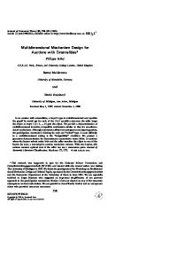
single-item only bidding can also lead to much longer auctions. The only redeeming feature of these auctions seems to be their revenue generating capabilities. Unfortunately, much of that revenue comes from losses to bidders as opposed to increased surplus extraction. This may be acceptable in the short run. However, if the design is used repeatedly, bidders will learn to avoid these losses, and efficiency and revenue will ultimately suffer. But we have gone further here than simply asserting that package bidding is sensible. We have provided a new auction design, RAD, which clearly outperforms others. Relative to the Milgrom FCC design, RAD produces higher efficiency, higher revenue, higher bidder profits and a much quicker time to completion. It even produces similar efficiencies to and higher revenues than the continuous AUSM with a standby queue. Since RAD uses a pricing rule instead of a queue to mitigate the threshold problem, it appears to be no more complex from a bidder’s point of view than the Milgrom auction and significantly simpler than the continuous AUSM. Finally, there is no evidence of degradation in performance when RAD is used in simple, additive environments. Why do we think RAD worked so well? We believe it is the decentralizing influence of the prices. Under the SIAM and Milgrom FCC mechanisms, prices were only calculated from single item bids. Therefore, if bidders were not bidding above their valuations, in this environment, it is guaranteed that the single item prices would be much lower than the actual winning bids for the packages. If we consider the sample parameters given in Table 2, the maximum prices for bidders unwilling to expose themselves to potential losses are: 3, 8, 2, 8, 16, and 9 for the first six items.37 The ‘competitive’ prices, however, are 38, 49, 30, 43, 38, and 49.38 If we examine the data for this parameter set (period 2), we find that this difference in prices is prevalent experimentally. Figure 5 lists the average prices under both SIAM and RAD. In general, the SIAM prices are closer to the zero exposure prices.39 The RAD prices are closer to the competitive prices. In general we would expect final prices to be somewhat lower than the competitive prices due to the bid increment requirement which made the true price higher than that reported here. Once the mandatory bid increment of three francs is considered, the RAD prices are not significantly different than the competitive prices for five of the six objects. In the RAD mechanism, prices are calculated using all bids. Therefore, in general, they will more closely represent the level of competition for an item. Since the prices are typically calculated in order to indicate the level of competition below the winning packages, they can indicate to bidders markets where bidding is thin. Thus, prices should aid in finding an appropriate fit. 37

These are simply the maximal single item values. The only way prices under the SIAM and FCC designs could be higher is if a someone bid on a single item above their value. 38 Competitive prices are the set of prices which leave only one demander for each object. In other words, combinations of these prices are greater than or equal to valuations for all packages except the efficient ones. 39 The fact that the prices were often above the zero loss prices indicates that bidder were willing to make bids that could’ve led to losses. Their motivation may have been to use the single item bids in order to signal willingness to bid on an object in hopes of finding a ‘fit’ with another bidder.

24

Period 2 Final Prices 50 45 40 35 30 Competitive Prices

25

Zero Loss Prices Average SI Prices

20

Average PR Prices 15 10 5 0 a

b

c

d

e

f

Object

Figure 5: Average Final Prices – Period 2 It would seem that the RAD design would be a natural candidate for use as a multiobject iterative auction in its current form. However, in spite of the excellent performance in our tests, there are at least three problem areas that might be considered for redesign. The first, and simplest to fix, is a result of the eligibility rule. If bidders have budgets for items, they may find themselves bidding for and even winning items which have little value to them simply to preserve eligibility. While this problem has generally been recognized even when there is no package bidding, we know of no papers which purport to provide a solution. There is, nevertheless, a solution which is straight-forward: the use of “OR” bids in an iterative auction. Bidders would be allowed to place a bid saying “I bid $1000 for A,B and C OR I bid $800 for D and E”. The appropriate constraints would be added to the allocation problem (1) and the rest of the mechanism would be left as is. This could be done to the Milgrom FCC rules as well as to RAD and others. OR bids may appear to increase a bidder’s problem complexity a bit, but such bids do eliminate the anxiety and confusion raised by the need to find “safe places” to preserve eligibility. We have not tested the effect of adding OR bids to the RAD design, something which should clearly be done before our recommendation is adopted in practice. A second problem with the RAD design is that, although the pricing rule seems to guide and coordinate small bidders to solve the threshold problems, it can also orphan 25

some bidders at early stages even through they belong in the efficient allocation. An example will illustrate. Suppose in round 5 there are 4 bids submitted Table 10: bid # $ Items 1 99 ABC 2 75 AB 3 75 AC 4 75 BC Under the RAD design bid #1 wins and the prices40 are (Πc Πb P ic ) = (33, 33, 33). Now suppose there is a bidder who is willing to pay 30 for A. Had they bid 28 for A in round 5 they would have been a winning bid along with bid #4. But now they can’t bid since Πa > 30. This may lower efficiency. There are several features of RAD that work against such orphaning. First, if this bidder had bid in round 5, they would not have been orphaned. So aggressive participation helps. Second, suppose in round 6, bid #3 is not resubmitted, but 1,2, and 4 are. Then 1 still wins and Π = (24, 51, 24).41 If it gets to this stage our bidder for A can reenter the fray if they still have the eligibility to do so. Of course, if the auction stops in round 5, which it will if there are no additional new bids, it will end at an inefficient allocation. We do have an additional design feature to address this problem but will defer its explication until we have seriously tested it. The last potential problem with RAD could not arise in our laboratory tests but could arise if RAD were scaled up to be used in the field. In the lab we used 5 bidders and 10 items. In practice one could have thousands of items and thousands of bidders. Scaling up creates the real possibility that the allocation problem (1) could take a very long time42 to solve in any given round. So all the gains in time to complete would be lost because of the complexity of (1). There are a number of design changes that can address this problem including replacing (1) with a less ambitious target. We have not yet tested them experimentally but we consider this a prime area of future research.

40

Notice that these are not separating prices which is what causes a problem. These are separating prices. This also shows that prices are not necessarily monotonically increasing (since 24 < 33). The sum of prices, however, is. 42 One can create problems which would take weeks to solve on supercomputers. 41

26

Appendix A The Exposure and Threshold Problems In the design of multi-object auctions, two significant impediments to efficiency have been identified by theorists: exposure and thresholds. The exposure problem is an undesirable feature of auctions with no package bidding. It tends to disadvantage bidders wanting multiple items. The threshold problem is an undesirable feature of auctions with package bidding. It tends to disadvantage bidders wanting single items.

A.1

The Exposure Problem

The exposure problem is simple to understand.43 It arises from the non-existence of competitive prices because of the non-convexities created by complementarities. We use an example with three bidders and two objects. Table 11: Exposure Example Packages Bidder A B AB 1 a a 2a + b 2 a a 2a + c 3 d a a+d Assume a + b > d > a, and b > c. Then the efficient allocation gives AB to 1. How might bidding proceed with only single-item bids? Assume all bid increments are equal. We would expect prices to initially increase to PA = PB = a, marked 1 on Figure 6. If bidder 3 increases the bid on A to something greater than a, then bidders 1 and 2 must decide whether to bid above their stand alone values for A. If they don’t, the allocation will be something like 1 gets B and 3 gets A. This is inefficient, although one could not tell that simply from the prices PA > a and PB = a. If either 1 or 2 (or both) continue bidding, they become exposed to losses. The auction will proceed to point 2 where PA = PB = a + 2c . At this point bidder 2 will drop out. Should bidder 1 continue? If 1 does, then bidding proceeds to point 3 where PA = a+b− 2c and PB = a + 2c . At this point, if bidder 3 raises the bid on A, which 3 should do, 1 faces a dilema: drop out or continue. If bidder 1 drops out at point 3, then 1 only gets B and loses −(a − a − 2c ) = 2c . Bidder 3 gets A and the allocation is inefficient. But 1 can calculate that if he bids for A at a price less than a + b then 1 will lose less than 2c since a − PB < 2a + b − PB − PA whenever PA < a + b, no matter what 1 pays for B. So by continuing, 1 makes lower losses than by stopping. So unless 1 believes someone will rescue her by bidding for B, 1 should continue on to point 4. In this auction, the bidding will stop at point 3. Bidder 1 will 43

Examples can be found in Bykowsky et al. (1995) and Milgrom (1997).

27

Figure 6: Exposure Example

PB 6 @

@

@

a+b

@

@

@

@

@

@

@

@

@ @ @ @ @ @ k k @s 2 @s3-s @ @ 4k  1ks @ @ @ @  @ @ @ @ @ @ @ @ @ @ a d 62a + c 2a + b

@

a

a+b

-

PA

win AB, the efficient allocation, and 1 will profit by 2a + b − (a + 2c + d). Unfortunately, if d > a + b − 2c then this is a loss for bidder 1. Only the auctioneer makes money. The exposure problem is a potential pitfall for any participant for whom V (AB) > V (A) + V (B). V (AB) − A(B) is the maximum they would be willing to pay for A if they know they have B. V (AB) − V (A) is maximum they would be willing to pay for B if they have A. If these sum to more than V (AB), they are potentially vulnerable. Depending on how bidders react to the problem, stop at point 1 or continue, the auction can produce inefficiencies or losses, neither of which is particularly desirable. Some analysts may attempt to infer, from existing data, whether exposure was problem. However,notice that if participants never reveal their values there is no way for the analyst to know for sure after an auction is over that 1 even faced an exposure problem. Dropping out at point 1 is consistent with a world in which there are no synergies (b = 0). Staying in to point 4 is consistent with a world where b > a − d − 2c and 1 does not lose. It is also consistent with a world in which V (B) > a + 2c , V (A) > d and there are no synergies. It is easy to see that package bidding will cure the exposure the problem. At point 1, bidder 1 would bid only for AB. This would continue to point 2 where 1 wins and the action stops. 1 wins AB, the efficient outcome, and pays 2a + c.

28

A.2

The Threshold Problem

We have just seen that package bidding can help keep the exposure problem under control. Unfortunately package bidding creates its own problem: thresholds.44 The problem is easy to understand. We use an example from Milgrom (1997) with bidders, 2 items, and budget contraints.45 Table 12: Threshold Example Packages Bidder A B AB Budget 1 4 3 2 4 3 3 1+ 1+ 2+ 2 Table 13: Threshold Game 2 Raises by 1 Raises by 0 1/2 3/4 0 (0,0) (0,0) (3 14 , 2 12 ) 3 3 1/2 (0,0) (2 4 , 2 4 ) (2 34 , 2 12 ) 3/4 (2 12 , 3 12 ) (2 12 , 2 34 ) (2 12 , 2 12 ) Under package bidding we could arrive at a round of the auction in which 3 is the current high bidder, bidding 2 for AB and beating bids of 3/4 by 1 for A and 3/4 by 2 for B. If 1 and 2 know this then they have to decide whether to rebid and by how much. This yields a game that looks like Table 13 where (x,y) is (1’s profit, 2’s profit). There are 3 pure strategy Nash equilibria with raises of (0,3/4), (3/4,0), and (1/2, 1/2). In all equilibria the outcome is efficient. But there is a coordination problem: If 1 assumes (0,3/4) and 2 assumes (3/4, 0), they end up at (0,0) and lose. 3 wins the item, and an inefficient outcome occurs.46 Will this happen? If 1 and 2 are Bayesian game theorists interested only in the current stages the answer is yes. Suppose 2 believes 1’s value for A is VA1 ∼ [0, 4] and 1 believes 2’s value for B is VB2 ∼ [0, 4] and this is common knowledge. 1’s strategy is b1 (VA1 ) and 2’s is b2 (VB2 ). 1’s payoff is VA1 − b1 (VA1 ) if b1 (VA1 ) + b2 (VB2 ) ≥ 4 and is 0 otherwise. So 1’s expected utility is [VA1 − b1 ]P [b2 (vB2 ) ≥ 4 − b1 ] = [VA1 − b1 ][1 − F (4 − b1 )] 44

We originally identified this problem in Banks et al. (1989). Milgrom (1997) calls it the free rider problem. While this is catchy, it is inappropriate. Free riding was identified in public good problems where it is a dominant strategy not to contribute. The problem with package bidding is more appropriately identified with games with multiple equilibria, such as public goods with thresholds. Here there are no dominant strategies to overcome just a coordination problem. We have thus chosen the more appropriate name. 45 Milgrom (1997) uses this to analyze a proposed design for the FCC. That design is significantly different from the package bidding auction we propose in this paper and is also different from AUSM as tested in Banks et al. (1989) or Ledyard et al. (1997). 46 It is often the case that cheap talk can help here. That is certainly the finding in many public goods experiments with thresholds. See Ledyard (1995).

29

Assume VA1 and VB2 are distributed identically and independently and uniform on [0,4]. Then b1 = 12 VA1 , b2 = 12 VB2 are equilibrium strategies. It is easily possible that VA1 + VB2 > 2 +  > 2 > 12 (VA1 + VB2 ). 3 wins even though it is inefficient. Of course an iterative auction does not require a one time decision. It allows for a form of bargaining or coordination. Under complete information, with an activity rule and minimum increments one can easily construct reasonable strategies for 1 and 2 in our example where, to preserve eligibility, they constantly increase their bids by the minimum increment. Eventually they will displace 3 and win. Of course whether and how this happens depends crucially on the details of the auction.

A.3

Summary

Simultaneous auctions without package bidding can suffer from the exposure problem. This can cause either bidder losses or low efficiencies. Simultaneous auctions with package bidding can suffer from the threshold problem. This can cause low efficiencies. Neither is a fatal flaw but each raises the same question. Can an auction be designed to eliminate the problem? For example, the withdrawal rule in the FCC auctions was designed to minimize the exposure problem while retaining single-item bids.47 In this paper, we provide a new design to minimize the threshold problem while eliminating the exposure problem with package bids.

Appendix B

Resolving Price Ambiguity

In Section 3.2, we indicated that the RAD auction pricing algorithm (8) might not yield a unique price vector.48 We use the following routines to eliminate that ambiguity. Let g ∗ , Π∗ , and Z ∗ solve (8). If Z ∗ = 0 then go to problem (10) below. If Z ∗ > 0, let J ∗ = {j ∈ Lt | Z ∗ = g∗j }. If J ∗ = Lt then go to (10) below. Otherwise, min Z

Πt ,Z,g

Subject to

X X X

(9)

Πtk Xkj = pj for all bj = (pj , xj ) ∈ Wt

k∈K

Πtk Xkj + g ∗j = pj for all bj = (pji , xj ) ∈ J ∗

k∈K

Πtk Xkj + g j = pj for all bj = (pji , xj ) ∈ Lt \ J ∗

k∈K 47

See Porter (1997) for an analysis of the effect ofP a withdrawal rule. An alternative approximation would minimize j (g j )2 which would avoid iteration. We chose to stick with linear programs for computational simplicity and a desire to minimize the number of bids missed rather than the total size of the miss. 48

30

0 ≤ g j ≤ Z for all bj ∈ Lt \ J ∗ Πt ≥ 0. ˆ gˆ, Π ˆ be the solution to (9). If Zˆ = 0 go to 10 below. Otherwise, let Jˆ = {j | Zˆ = Let Z, j ∗ gˆ }. If J ∪ Jˆ = Lt then go to problem (10) below. Otherwise, let J ∗ = J ∗ ∪ Jˆ and go to (9) again. When the iteration on (9) is complete we will have prices which approximate our “ideal” but not always obtainable prices. They may still not be unique. So, we go through a sequence of iterations which eliminate non-uniqueness and which create prices ˆ gˆ, Π ˆ be the solution from the last to guide bidders to solve the threshold problem. Let Z, ˆ = K. iteration of (9). Let K max Y (10) subject to X X k∈K

Πtk xjk = pj for all (pj , xj ) ∈ Wt

k∈K

Πtk xjk + g j = pj for all (pj , xj ) ∈ Lt ˆ Πtk ≥ Y for all k ∈ K.

(11)

˜ =K ˆ \ K ∗ . If K ˜ = 6 ∅, return Let Y ∗ , Π∗ solve (10). Let K ∗ = {k ∈ K | Πtk = Y ∗ }. Let K to (10) and solve it replacing (11) with ˜ Πtk ≥ Y for all k ∈ K ˜ Πtk = Π∗t k for all k ∈ K \ K. ˜ = ∅, we are done and the prices Π∗ = Πt+1 . These are unique, approximate the When K ideal prices, and provide signals about thresholds.

Appendix C

Instructions

You are about to participate in an economics experiment in which you will earn money based on the decisions you make. All earnings you make in the experiment are yours to keep. 1. All values and prices will be stated in francs. Each franc you earn can be converted into US currency at the rate specified on your Redemption Value Sheet. 2. We will be conducting a market in which you can buy any of the 10 items. You can only buy the items–not sell them. The items are denoted A-J. 3. The market will be broken up into a series of rounds. You only earn francs when the market closes, not for each round. 31

4. When the market closes you will fill out your Accounting Sheet and a monitor will verify your earnings. The experiment may have more than one period. Each period will consist of a series of rounds. During each round you may bid on items. At the end of each round, the high bid for each item will be displayed to everyone. The bidder with the highest bid for each item is the temporary winner of that item. After the successful bids are displayed, a new round will begin during which you may choose to try to gain or maintain ownership of any item. We will continue this process until the temporary ownership of each item remains the same for 2 rounds.

C.1

Redemption Value Sheet

You will have a redemption value sheet for each period in the experiment. This sheet lists your values for each of the items A-J. Your values are private information. Please do not reveal them to anyone. At the end of the period the owner of each item will receive francs for the amount of their value of the owned item, less the amount that was bid for that item in the last round of the period. For example, If Bidder 3 has a redemption value sheet of A 17 B 36 C 22 and Bidder 3 had the highest bid for item B in the last round with the high bid = 30 francs, then Bidder 3 will receive 6 francs for the period. For each new period you will receive a new redemption value sheet. Your values and your conversion rate may change.

C.2

Submitting an Order

You submit bids in the ’Make a Bid’ window. You select the item(s) you would like to bid on, and indicate the amount that you wish to bid for the item(s). You may submit a bid for a single item, for example, A= 100. You may also submit bids for multiple items at the same time, for example, ABC=200. This would mean 200 for owning all three items, it is not a bid of 200 for each individual item. You may make as many bids in each round as your eligibility permits.

32

C.3

Eligibility

To encourage active bidding there is a ”use it or lose it” rule. In the first round you can bid for any and all items. In each subsequent round, you will be allowed to bid only on as many items you had active bids on in the previous round. An active bid is any bid that is considered by the solver in computing the solution of that round. It is a standing bid (a high bid from the last round) or a newly placed bid. The maximum number of items you are allowed to have in all of your active bids in a round is called your eligibility. Thus, your eligibility at the beginning of the period is 10. Your eligibility in round 12 is exactly the number of items in your active bids in round 11. How is eligibility computed? Suppose that at the end of round 1 you had one high bid in the solution: A=50. Further you had submitted 2 more bids of B=43 and C=17 which did not become high bids. You did not bid on any other items. Your eligibility in round 2 will be 3. This means that you can bid on a total of 3 items in round 2. Your eligibility will be displayed in the round results. The computer would indicate that you have a free eligibility of 2 and that you have a high bid eligibility of 1. You may use the 1 unit of high bid eligibility to bid on item A. If you do not increase your bid for A you will not lose this part of your eligibility in round 2. Either you will still have the high bid and retain the 1 unit or someone will beat your high bid and you will be given a normal unit of eligibility for round 3. Your 2 units of free eligibility can be used on any other items. The computer will indicate that you may use these 2 units on items: B C D E F G H I J. Note, you are not limited to selecting items B and C to use your eligibility. You may choose any 2 items for which to submit bids. So a person with the above described eligibility might choose to submit bids like: Bid Bid Bid Bid Bid

1: 2: 3: 4: 5:

A=60 CG=75 CA=52 ACG=100 C=90

Notice that even though you had eligibility of 3, you are able to submit any number of bids. Eligibility only limits the number of items you may bid on, not the number of bids that you may submit.

33

C.4

The Solver

At the end of each round the solver will determine which bids are the temporary winning bids. The solver selects the combination of bids which maximize the revenue to be received. Example: At the end of round 1 the following bids have been submitted: Bid 1: ABC = 200 Bid 2: A = 100 Bid 3: BC = 75 The temporary winning bid is, therefore, bid 1 since it beats 100+75 for A + BC. In round 2 a participant who wants only AB can submit a bid of 150 for AB in hopes that someone else will bid 51 or greater for item C. The solver would realize that these two separate bids are greater than the bid for ABC even when the bids come from different participants. If you have a temporary winning bid at the end of a round, that bid will automatically be resubmitted into the next rounds bids. You may not withdraw a temporary winning bid. You do not need to resubmit that exact bid, although you have the option of beating your own bid.

C.5

The Calculation of Prices

While the computer is calculating the temporary winning bids, it will also compute prices for each item. These prices will determine the minimum prices in the next round. The computer will first try to calculate prices, one for each item, so they sum up to the standing bids and are greater than any second highest bid. Example 1: Bid 1: A=30 Bid 2: B=10 Bid 3: C=21

prices

a 30

b 10

c 21

Example 2: Bid 1: AB=30 a b c Bid 2: C=8 prices 15 15 9 Bid 3: ABC=39 The standing bid is number 3 for ABC. Choosing it yields the highest revenue. The 34

computer will calculate prices for items A,B,C that add up to 39 and so the prices for A and B add up to at least 30 and the price of C is at least 8. If there are several possible solutions then the computer will try to equalize the prices. Example 3: Bid 1: AB=30 a b c Bid 2: BC=30 prices 13 13 13 Bid 3: AC=30 Bid 4: ABC=39 Here bid number 4 is the only standing bid. Following the rules we would need to find prices for ABC that add up to 39. But we also want the prices for A and B to add up to at least 30, the prices for A and C to add to at least 30, and the prices for B and C to add to at least 30. But that is not possible. When this happens, the computer will find prices that come as close as possible to meeting the rules. So it is possible that you will have a bid that exceeds the minimum prices and yet is not a winning bid.

C.6

Minimum Bids

At the start of each round, a price for each item will be displayed by the computer. Your bid for any package must be greater than the summation of the posted prices for each item plus 3 francs for each item in the bid. For example, suppose that prices are: a b c prices 10 23 176 Some bids that meet the minimum requirements are: Bid 1: A=14 Bid 2: B=27 Bid 3: BC=206

C.7

Round Results

All the information that you need to make decisions in the second round and beyond will be displayed in the round results. (It might be a good idea to keep an eye on your valuation sheet as well.) At the end of each round the computer will make all of the necessary calculations. The experiment monitor will let you know when the results are ready.

C.8

Bids Button

You can see your bids while the round is active.

35

You can only see the bids for the current round and, again, you can only see your own. The information you get will look like this: Bidder B# P R $ a b c d e f g h i j two 211 0 3 600 1 From now on you are all identified by your bidder number. Each bid is assigned a unique bid ID. This is in the B# column. ’P’ is the period and ’R’ is the round in which that bid was submitted. Under the dollar sign is the amount of the bid in francs. For each of the items (A-J) there will be either a one or nothing. A one means that the item is part of the package being bid for.

C.9

Stopping the Market

Each market will consist of a series of rounds. Each round will be no greater than two minutes in length. The period will be closed at the end of round T if there is no change in the temporary ownership between the end of round T-1 and the end of round T.

C.10

Special Notes

All bids must be in whole numbers (increments of size 1). In general, you will probably discover a few menu options that have been grayed out. You will not be able to use these options during this experiment. If the bidding and trade windows disappear, you may type in the remaining window with writing and return to restart the program. A login screen will appear. Type your bidder number spelled out as your name (i.e. “one”) and type the number “0” as your password, then click on done. Your bidding and trade windows should reappear. If you have any problems, please ask for assistance. We do not offer any guarantees that the software will not crash. When the computer crashes there may be some excitement, but there is no need to panic. The first few rounds will be practice rounds. Participants should learn and ask questions during this period.

References Armstrong, M. 1998. Optimal multi-object auctions. Unpublished. Ausubel, L. M. 1997. An efficient ascending-bid auction for multiple objects. Working Paper 97-06, University of Maryland, College Park, MD. 36

Ausubel, L. M. and P. Cramton. 1998. Auctioning securities. Unpublished. Banks, J. S., J. O. Ledyard, and D. P. Porter. 1989. Allocating uncertain and unresponsive resources: an experimental approach. Rand Journal of Economics 20(1):1–25. Bikhchandani, S. and J. M. Ostroy. 1998. The package assignment model. Unpublished. Bykowsky, M. M., R. J. Cull, and J. O. Ledyard. 1995. Mutually destructive bidding: The FCC auction problem. Social Science Working Paper 916, California Institute of Technology, Pasadena, CA. Cramton, P. C. and J. Schwartz. 1998. Collusive bidding: Lessons from the FCC spectrum auctions. Forthcoming in Journal of Regulatory Economics. Engelbrecht-Wiggans, R. and C. M. Kahn. 1998. Multi-unit auctions with uniform prices. Economic Theory 12:227–258. Ferejohn, J., R. Forsythe, and R. Noll. 1979. An experimental analysis of decision making procedures for discrete public goods: A case study of a problem in institutional design. In Smith, V. L., ed., Research in Experimental Economics, volume 1, pages 1–58. JAI Press. Grether, D., M. Isaac, and C. Plott. 1981. The allocation of landing rights by unanimity among competitors. American Economic Review 71:166–171. G¨ ul, F. and E. Stacchetti. 1995. English auctions with multiple goods. Unpublished. Hurwicz, L. 1960. Optimality and informational efficiency in resource allocation processes. In Proceedings of a Symposium on Mathematical Methods in the Social Sciences, 1959, pages 27–46, Stanford. Stanford University Press. Ishikida, T., J. Ledyard, M. Olson, and D. Porter. 1998. Implementation of a combinatorial market: The experiments behind the automated (environmental) credit exchange (ACE). Unpublished. Kagel, J. H., R. M. Harstad, and D. Levin. 1987. Information impact and allocation rules in auctions with affiliated private values: A laboratory study. Econometrica 55:1275– 1304. Kwasnica, A. M., J. O. Ledyard, D. Porter, and J. Scott. 1998. The design of multiobject multi-round auctions. Social Science Working Paper 1045, California Institute of Technology, Pasadena, CA. Forthcoming. Ledyard, J. O. 1995. Public goods: A survey of experimental research. In Kagel, J. H. and A. E. Roth, eds., The Handbook of Experimental Economics, chapter 2, pages 111–194. Princeton University Press, Princeton, New Jersey. Ledyard, J. O., D. Porter, and A. Rangel. 1997. Experiments testing multiobject allocation mechanisms. Journal of Economics and Management Strategy 6:639–675. 37

Milgrom, P. R. 1995. Auctioning the radio spectrum. In Auction Theory for Privitization, chapter 1. Cambridge University Press. Milgrom, P. R. 1997. Putting auction theory to work: The simultaneous ascending auction. Unpublished. Milgrom, P. R. and R. J. Weber. 1982. A theory of auctions and competitive bidding. Econometrica 50(5):1089–1122. Myerson, R. B. 1981. Optimal auction design. Mathematics of Operations Research 6:58–73. Noussair, C. 1995. Equilibria in a multi-object uniform price sealed bid auction with multi-unit demands. Economic Theory 5:337–351. Plott, C. R. 1997. Laboratory experimental testbeds: Applications to the PCS auction. Journal of Economics & Management Strategy 6:605 – 638. Porter, D. P. 1997. The effect of bid withdrawl in a multi-object auction. Social Science Working Paper 982, California Institute of Technology, Pasadena, CA. Rassenti, S. J., V. L. Smith, and R. L. Bulfin. 1982. A combinatorial auction mechanism for airport time slot allocation. Bell Journal of Economics 13:402–417. Riley, J. G. and W. F. Samuelson. 1981. Optimal auctions. American Economic Review 71(3):381–392. Smith, V. L. 1979. Incentive compatible experimental processes for the provision of public goods. In Smith, V. L., ed., Research in Experimental Economics, volume 1, pages 59–168. JAI Press. Smith, V. L. 1982. Microeconomic systems as an experimental science. American Economic Review 72:923–955. Vickery, W. 1961. Counterspeculation, auctions, and competitive sealed tenders. Journal of Finance 16:8–37. Williams, S. 1994. A characterization of efficient bayesian incentive compatible mechanisms. Math Center Working Paper 1100, Northwestern University, Evanston, IL. Forthcoming in Economic Theory.

38