Ali Ahmadinia, Christophe Bobda, Marcus Bednara , Jürgen Teich. Department of Computer Science 12. University of Erlangen-Nuremberg, Germany.
A New Approach for On-line Placement on Reconfigurable Devices∗ Ali Ahmadinia, Christophe Bobda, Marcus Bednara , J¨urgen Teich Department of Computer Science 12 University of Erlangen-Nuremberg, Germany {ahmadinia,bobda,bednara,teich}@cs.fau.de Abstract By increasing the amount of resources on reconfigurable platforms with the abililty of partial reconfigurability, the issues of the management of these resources and their sharing among different tasks will become more of a concern. Online placement is one of these management issues that is investigated in this paper. Here we present a new approach for online placement of modules on reconfigurable devices, by managing the occupied space rather the free space on the device. Also an optimization of communication between running modules themselves and outside of the chip is proposed. The experimental results show a considerable decrease in communication and routing costs.
1 Introduction Modern reconfigurable devices allow reconfiguration of a part of the device while the rest remains unchanged. This allows tasks to be allocated on parts of the space of the reconfigurable device for their execution at run-time. Runtime space allocation, also known as temporal placement or on-line placement is a central part in reconfigurable computing. Unfortunately, much research was not dedicated to this purpose. This is partly due to the fact that manufacturers of reconfigurable device currently do not provide devices with unlimited partial reconfiguration capabilities as well as tools for partial reconfiguration. As such devices begin to appear on the market, a strong investigation of online placement is needed. For the on-line placement problems, two subproblems have to be solved in order to place a ready to execute task: 1. Identifying the set of potential sites to place the new task. 2. Selecting the best site to place the component according to a set of given criteria. ∗ Supported in part by the German Science Foundation (DFG), SPP 1148 (Rekonfigurierbare Rechensysteme).
Most of the work on on-line placement [1][2][3] uses a free space manager to solve subproblem 1. The free space on the device is represented as a set of empty rectangles. For an incoming component, one of the empty rectangles is chosen according to the placement strategy (best-fit, first-fit, etc...) , the task is placed inside the chosen rectangle and the new set of empty rectangles is computed. The main drawback of this method (free space segmentation) is that the set of empty rectangles increases very fast each time a new task is placed, thus making the search for a suitable site (subproblem 2) difficult. Moreover, incoming tasks are handled as independent entities. Therefore the communication aspect is neglected. In this paper, we present our new approach for on-line placement of components on reconfigurable devices. It exploits the fact that the set of empty rectangles grows much faster than the set of placed rectangles (tasks) and therefore it is more suitable to manage the occupied space rather than the free space on the device. In real application each task communicates somehow with its environment. This communication is done in form of inputs to and outputs from the tasks. Therefore communication among tasks plays an important role in our placement strategy. The optimization of the communication is an important criterion in finding the solution of subproblem 2. The organization of the paper is as follows: Section 2 gives the formal definitions of the on-line placement problem. Section 3 explains the on-line placement algorithm. Section 4 describes the implementation of our on-line placement approach. In Section 5 we do some evaluations of our method and we conclude the paper in Section 6.
2 Background and Definitions Before explaining the online placement problem, the definitions and assumptions of our system model according to the related work in this area will be given. We assume that a reconfigurable device R is made upon a set of reconfigurable Processing Elements (PE) arranged in rectangular array with H rows and W columns. The PEs can
be somehow connected together. Our model of dynamic reconfiguration is made upon a scheduler, an on-line placer and the reconfigurable device (Figure 1). The scheduler manages the tasks and decides when a task should be executed. Then the task is given to the placer which will try to place it on the device, i.e allocating a set of PEs for that task. If the placer is not able to find a site for the new task, then it will be sent back to the the scheduler which can decide to send it later or to send another task to the placer. In this case, we say that the task is rejected. The development of a scheduler is not in the scope of this work. We are interested in the development of the placer part of our system. For each task to be placed on a
• ek is execution time of task tk • wk is width of the corresponding module for task tk in terms of PE • hk is height of the corresponding module for task tk in terms of PE We set tk = (ak , ek , wk , hk ) The arrival time of a task is the time when the placer receives the task from the scheduler, and it is independent from if the task is placed or rejected. At each point in time, the placer contains a Dynamic Set of Tasks that we call it DST. The DST consists of the running tasks and the new task to be placed on the device. Elements are dynamically inserted and removed from the DST. Also we assume that tasks are non-preemptive because of high configuration overhead. Although this assumption does not influence out placement approach. Running modules are also non-replaceable. Since we are interested in the communication among tasks and their environments, we will not consider only connections among different tasks, but also connections between tasks and the boundary of the device. This is usefull for tasks which have an off-chip communication. For a given DST, we define a dynamic set of of connections (DSC). An element of the DSC is either a connection among two tasks or a connection among one task and a location on the boundary device. Definition 2 (Task Communication) Given a dynamic set of tasks (DST) T and a set of positions (pins) P on the boundary of reconfigurable device R. We define the dynamic set of communication (DSC) C as the set of edges between T and (T ∪ P). The weight w pq of an edge (p, q) ∈ C is the width of the bus connecting the two elements p ∈ T and q ∈ (T ∪ P).
Figure 1. A multitasking sytem on reconfigurable device reconfigurable device, we further assume that an implementation as a rectangular block is available with the inputs and output ports on its boundary. This implementation is stored in a module database, and will be retrieved on demand. We define the characteristics of a task as follows: Definition 1 (Task Characteristics) Given a set of tasks T = {t1 ,t2 , ...,tm }. The characteristic of a task tk ∈ T is 4-tupel (ak , ek , wk , hk ) where • ak is arrival time of task tk
Having defined the task characteristics, the DST and the DSC, we explain in the next sections how our online placement algorithm works.
3 Algorithms 3.1 Space Manager As mentioned in the introduction, the first part of the placement problem is to identify all possible sites where a new module can be placed. The easiest way to solve this subproblem is to use a Brute Force Algorithm. For each new component c to be placed, the Brute Force Algorithm solves the first subproblem by scanning all the positions on the device. For each position p = (x p , y p ), it checks if an overlapping will occur between
c and a placed module, if the component c is placed at location p. Having solved subproblem 1, the optimal placement position is computed by computing the placement cost for each of the locations found in the first step and select the best one as the optimal solution. The Brute force requires O(H × W × n) time to solve subproblem 1. H is the height, W the width of the reconfigurable device and n is the number of running tasks on the hardware. Bazargan et al. [1] proposed to store only the free spaces as maximal rectangles, however the complexity of this approach is O(n2 ). For large reconfigurable devices, H and W are greater than n, thus making the Bazargan approach better than the Brute Force approach. However, in Bazargan’s approach, a binary tree is used for managing empty rectangles, which is complicated to keep updated by deletion and insertion of modules, because in some cases many nodes of the tree have to be changed. Hence we propose a simpler and faster approach with complexity of O(n). Contrary to the Bazargan’s approach, we propose to manage the occupied space of the device rather than the free space. Our approach is based on the observation that the set of empty rectangles on the device grows much faster than the set of placed components, therefore it will be much faster to use the occupied space to find the set of free sites where the new component can be placed. Without loss of generality, we will consider that components are placed relatively to their lower left positions. We first define the impossible placement region (IPR) for a new component. Definition 3 (IPR relative to placed modules) For a new component c to be placed on the device and a placed component c0 , the Impossible Placement Region (IPR) Ic0 (c) of c relative to c0 is the region where c cannot be placed without overlapping with c0 . For a set C0 of placed components, the impossible placement region IC0 (c) of c is the region where c cannot be placed without overlapping with an element of S C0 : IC0 (c) = c0 ∈C0 Ic0 (c).
Definition 4 (IPR relative to the device) The Impossible Placement Region IR (c) relative to the device is the region of the device where c cannot be placed without overlapping with the external area of the device.
Definition 5 (Impossible and Possible Placement Regions) The IPR for a new component c is identified by IC0 (c) and IR (c): I(c) = IC0 (c) ∪ IR (c) The possible placement region (PPR) P(c) of c is obtained by subtracting the IPRs of the running components and that of the device from the device area. If U is the set of all locations on the device, then P(c) = U − I(c).
For a new component c with height hc and width wc to be placed on the device and a placed component c0 , the Impossible Placement Region (IPR) Ic0 (c) of c relative to c0 is identified by computing the left margin with size hc − 1 and the bottom margin with size wc − 1 of the component c0 as illustrated in figure 2. By integrating this margin and the area of its running task,
Figure 2. IPR of a new module relative to a placed one we will have the impossible area for placing the new module, which is arisen by this running task. Then these margins should be defined for all runnig modules to have the impossible area arised from all placed modules. Also there exist two margins for the border of the reconfiguable device. It is obvious that the margins for each placed module must be recomputed as a new module arrives for placement. Computing the IPR relative to the device and each placed component as described before gives us the set of IPRs as shown in figure 3. The solution of subproblem 1 can be obtained by set subtracting the IPRs from the total device area. Since we have to compute the extended margins for the running modules and two regions relative to the device for solving the subproblem 1, the required steps of our algorithm is O(n).
3.2 Fitter The second subproblem in online placement is to find the optimal position for placing the new module from the set of possible placement regions. A simple approach consists of scanning all the possible placement positions, and
((x j +
wj 2
− xi − w2i )2 + (y j +
hj 2
− yi − h2i )2 ) × wi j
In other words, the routing cost between two modules is the weighted distance between them. In order to compute the routing cost we use the center point of the components instead of using the bottom left corner point as the reference point. For module i, this is defined by the pair (xi + wi /2, y + hi /2) where (xi , yi ) define the lower left position of i, wi the width and hi the height of i . If there is no communication between two modules Pi , Pj , the wi j and also the routing cost between them will be zero. When we have (n − 1) placed modules, and we want to place the n-th module, then we should minimize the routing cost of this module to all other placed ones. According to the definition 6, this corresponds to equation 1: n−1
min{ ∑ (((xn + i=1
Figure 3. The area of impossible positions for the new module
computing the placement cost for each position and then selection of the optimal one. This straightforward but ineficient approach requires O(|PPR| ∗ n) where n is the number of placed components. The Brute Force method is therefore too costly for an online placement algorithm. Instead of computing the placement cost for each point and selecting the best one, we will first compute the point popt which gives us the optimal placement cost. If popt is located within the PPR then we have the solution of subproblem 2. Otherwise, we will look for the closest point to popt which is located in the PPR and select it as the optimal placement position. For definiton of optimal point, we will first define our cost function, which should be minimized by the optimal point. One of the most important cost functions is routing cost. Then our main goal here is to place the components in such a way that the communication among components is optimal. This goal can be reached by placing connected components nearby each other. Furthermore, components which have off-chip connections should also be placed on the boundary of the device, not far from the pins that they use. We define the cost to minimize as the communication cost among the components placed on the device in terms of distance and buswidth. We call this cost the routing cost and formally define it as follows: Definition 6 (Routing Cost) For two modules i and j, we define the routing cost between modules i and j as follows: RoutingCost(Ri j ) =
wn wi hn hi − xi − )2 + (yn + − yi − )2 ) × win )} 2 2 2 2 (1)
In Equation 1, xn and yn are variables and other parameters are fixed. As xn and yn are independent of each other, equation 1 can be written as equation 2 and equation 3: n−1
min{ ∑ ((xn + i=1
n−1
min{ ∑ ((yn + i=1
wi wn − xi − )2 × win )} 2 2
(2)
hn hi − yi − )2 ) × win )} 2 2
(3)
The value in equation 2 is a function of xn , then for minimizing we should find in which point the partial derivative of this function for xn is zero, that means: wi 2 wn ∂{∑n−1 i=1 ((xn + 2 − xi − 2 ) × win )} =0 ∂xn
(4)
Therefore, the optimal value of xn is: xn =
wi wn ∑n−1 i=1 win (xi + 2 − 2 ) ∑n−1 i=1 win
(5)
In a similar way, we can compute the optimal value for yn : yn =
hi hn ∑n−1 i=1 win (yi + 2 − 2 ) ∑n−1 i=1 win
(6)
After finding the optimal point for placing the new module, the point must be checked if it belongs to the PPR set. In the case that the point is not located in the PPR set, we will find the Nearest Possible Position (NPP) to the optimal point. As shown in Figure 4, there are four nearest points out of the IPR, that the closest one will be selected as the
Figure 4. Near possible points to the optimal point
NPP. If also this point is not feasible, the former step will be repeated until the nearest feasible one to be found. Figure 5 shows the impossible areas which cover the optimal point and how the near possible points are tried to be identified. To find the NPP, a list of near possible positions according to the each overlapping area is used. In the worst case all the impossible areas cover this optimal point and the number of points in the list will be O(n), then NPP can be computed in O(n) time. The steps of the algorithm of NPP is as follows: Compute-OptimalPoint(new component) if OptimalPoint is feasible then place the component at the optimal point else NPP-Compute: 1. Find the 4 near points outside the margin, which the selected point is located. 2. Insert these points to the optimal points list. 3. Select the closest point to the optimal point from the near points list. 4. If the selected point is feasible then place the component at the optimal point else remove it from the near points list, and repeat NPPCompute step.
4 Implementation For implementing our online placement approach, we use a linked-list of size O(n) (for n running tasks) to store the placed and running modules on the reconfigurable device. The second structure which has been used is a twodimensional matrix with the same dimension of the reconfigurable device. This matrix represents the total status of the device, such that each element of it gives the status of one PE. It means when a point (PE) is occupied by a mod-
Figure 5. Near possible points to the optimal point
ule, the corresponding element in the matrix will have a pointer to the related module. Otherwise, the point in the matrix shows the emptiness of the point. Also for identifying PPR, the effects of extending and deleting margins will be applied on this matrix. Using the matrix allows to access each element and obtain its status in just one computing step. The other alternative data structure which needs less memory is using linked-list. But in this case, we have to parse the running module list for obtaining the status of each element, and its complexity is O(n) in each step. As mentioned before we use here the matrix, hence the computation is done faster. Another data structure of our implementation is a dynamic two-dimensional matrix which shows the communication bandwidths between each pair of running modules. The size of its dimensions are the same as the number of running tasks. This communication matrix is used for choosing the best position for placing a new module, because we need the communcation widths to compute and minimize the routing cost of placing new module. For finding optimal or near optimal point for placing a new module, we use a linked list for saving near optimal points. Always the nearest point to the optimal point from this list will be selected, and this point will be checked in the mentioned matrix, if it is a feasible position or not. If it is so then we have the NPP, otherwise this point is occupied by a running module or its margin. Then the nearest points, out of each border of the running module will be inserted to this list, and the selected point will be removed. Also in this list,
the trace of our search will be stored, because to be sure not to select a near point in a running module which has covered a prior near selected point. As mentioned before, in the worst case, we will have 3n near points in this list, therefore computing the NPP is O(n).
BF, because it has more space to find an optimal position.
5 Evaluation As we mentioned before, the complexity of our space manager is O(n), but for the KAMER (Bazargan’s method), it is O(n2 ) [1]. Therefore our space manager is faster. About the fitter, contrast to related work, instead of using a heuristic method, we try to optimize the defined routing cost function. To investigate the influence of our proposed method for Figure 7. The routing cost for different fitters (task size : [20,30])
Figure 6. The routing cost for different fitters (task size : [20,40]): Nearest Possible Position (NPP), First Fit (FF), Best Fit (BF) the Fitter, we have implemented a system model, with randomly generated task sets. This was done for different task sizes and shapes, precisely for tasks with width and height uniformly distributed in different intervals. To see the behaviour of algorithm with very different sizes of tasks, intervals of [20,40] (Figure 6),and [20,30] (Figure 7), and also to observe the behaviour for nearly square shaped tasks [25,30] range (Figure 8) has been used. The size of chip has been assumed 56x84 and 80x120, a 2-dimensional PE array, similar to the Xilinx Virtex XCV800 and XCV2000E FPGA devices, respectively. As depicted in the following figures, our method is compared with First Fit (FF) and Best Fit (BF) methods. Our method gives the least costs and BF gives the most routing cost. The FF method in the case of nearly square tasks reaches a comparable result to our method, but in all cases needs more costs for routing.On the other side, FF behaves much better than the BF in communcation costs. Also when we use a larger chip size, our fitter works better than FF and
Figure 8. The routing cost for different fitters (task size : [25,30])
6 Conclusion In this paper we have discussed existing online placement techniques for reconfigurable devices. We suggested a new space manager and fitter for online placement. In contrast to other approaches, our space manager keeps the information of occupied space instead of free space. This space manager has the best quality like KAMER [1], but it is faster. We have also taken into account the communication of tasks in the fitter, which was not cared before. We have conducted experiments to evaluate our fitter algorithm and existing ones. We reported on simulations that show a high improvement on the communication cost compared to [1]. Concerning future work, we plan to develop
a framework, that allows a designer for an efficient module implementation with respect to temporal placement and simulation of communication costs. Furthurmore, we will analyze our approach for its suitability to be implemented in an embedded system environment.
References [1] K. Bazargan, R. Kastner, and M. Sarrafzadeh. Fast Template Placement for Reconfigurable Computing Systems. In IEEE Design and Test of Computers, volume17, pages 68-83, 2000. [2] A. Ahmadinia, and J. Teich. Speeding up Online Placement for XILINX FPGAs by Reducing Configuration Overhead. To appear in Proceedings of 12th IFIP VLSI-SOC, December 2003. [3] H. Walder, C. Steiger, and M. Platzner. Fast Online Task Placement on FPGAs: Free Space Partitioning and 2-D Hashing. In Proceedings of Reconfigurable Architectures Workshop (RAW). IEEE-CS Press, April 2003. [4] Grant Wigley, and David Kearney, Research Issues in Operating Systems for Reconfigurable Computing, In Proceedings of the 2nd International Conference on Engineering of Reconfigurable Systems and Architectures (ERSA). CSREA Press, June 2002. [5] Oliver Diessel and Hossam ElGindy, On scheduling dynamic FPGA reconfigurations, In Kenneth A Hawick and Heath A James, eds, Proceedings of Australasian Conference on Parallel and Real-Time Systems (PART) , pp. 191 - 200, 1998, Springer-Verlag. [6] S´andor Fekete, Ekkehard K¨ohler, and J¨urgen Teich, Optimal FPGA Module Placement with Temporal Precedence Constraints, In Proc. of Design Automation and Test in Europe , IEEE-CS Press, 2001, pp. 658-665.