Apr 23, 2010 - [7] Kennedy, J. and Eberhart, R.: Particle swarm optimization, Proc. ... [10] Liang, J. J., Suganthan, P. N., Deb, K.: Novel composition test ...
Apr 23, 2010 - The loudness also varies from the loudest when searching ... the time difference between their two ears, and the loudness variations of the.
Apr 4, 2013 - The SCP is NP hard in the strong .... The first approach uses a repair heuristic to transform ... region, the cost minimization objective drives the.
Search is used as the main search algorithm, a Genetic Algorithm is in charge with the diversi cation ..... no one is using the console . The implementation of the ...
... have been ap- plied with some success to the Unit Commitment (UC) prob- lem. ... problem (due to important start-up and shut-down costs) the UC problem is ...
Feb 22, 2014 - Automation in a packing system saves much economic ... Institute of Technology Indore, Indore, ... The fast growing economy of countries in.
Other implementation are of HMAs are such as a ... HMAs for the solution of engineering problems. The WTO ...... Programming Recipesâ, Melbourne, 2011. [51].
Oct 21, 2011 - Internet hosting centers, which was followed by the development of a novel bee algorithm by D. T. Pham et al. in 2005 and the artiï¬cial bee ...
circuit board fabrication [10], ceramic tile manufacturing [11], and lead frame manufacturing [12]. There is a considerable amount of research available for the.
Abstract: We solve a linear chance constrained portfolio optimization problem using. Robust Optimization (RO) method wherein financial script/asset loss return ...
Mar 9, 2014 - rial equation for machine tool space description is presented. The development of ... compared with three other popular metaheuristics: classic.
search method, the Ant Colony Algorithms, particle swarm optimization (PSO) .... several improvements have been proposed such as: organic operators, elitist ...
Nov 15, 2013 - sessment protocol proposed by Knowles et al. [26]. Such a way ..... Theory of NP-Completeness, W. H. Freeman & Co Ltd, 1979. [8] E. Boros ...
Oct 21, 2011 - derivatives accurately, and thus derivativeâfree algorithms such as .... Internet hosting centers, which was followed by the development of a ...
the cycle of forming predicted behaviours and computing the control history ...... inequality design approach of robust PID controller with two degrees of freedom ...
Sep 28, 2016 - the following simulation conditions: 1. ... Or scatter of random subjective RR was narrowed to 30%-70% value corridor. ... candidate to overcome major drawbacks of traditional BPM as there are deviations of lived processes ... Foundati
Downloaded from De Gruyter Online at 09/28/2016 10:33:18PM via free .... of its competitors' devices is limited while Samsung products are readily available.
placement step of the VLSI physical design stage is a multiobjective optimization .... lack of compensation of t-norm for any partial fulfillment and complete sub-.
http://www.ing.unlp.edu.ar/cetad/mos/memetic_home.html. ⢠Evolutionary .... Example â A student has a choice between two courses, one in AI and one in OS.
Jul 12, 2014 - Carlos A. Coello Coello, Vincenzo Cutello, Kalyanmoy. Deb, Stephanie Forrest, Giuseppe Nicosia, and Mario. Pavone, editors, Parallel ...
British Standards BS5950. Saka [127] used genetic algorithm in the minimum design of grillage systems subjected to deflection limitations and allowable stress ...
May 29, 2015 - Volume 9121 of the series Lecture Notes in Computer Science pp 269- ... The Flexible Job Shop scheduling Problem (FJSP) is an extension of ...
Nov 6, 2012 - ing HPC Applications on a Geographically Distributed Cloud Federation. Journal of Cluster. Computing, Springer, 2012. .
Applicationsâ, John Wiley, 2010. [11] S. Luke,. âEssentials of .... [43] G. Venter, J. Sobieszczanski-Sobieski, âMultidisciplinary Optimization of a. Transport Aircraft ...
Sep 13, 2017 - [17] G. Venter and J. Sobieszczanski-Sobieski, âParticle swarm opti- mization ... through Simulated Evolution, John Wiley, New York, NY, USA,.
Hindawi Mathematical Problems in Engineering Volume 2017, Article ID 6043109, 15 pages https://doi.org/10.1155/2017/6043109
1. Introduction Nowadays in the economic-competitive world, optimisation has become increasingly popular for real applications as it is a powerful mathematical tool for solving a wide range of engineering design types. Once an optimisation problem is posed, one of the most important elements in the optimisation process is an optimisation method or an optimiser used to find the optimum solution. Optimisers can be categorised as the methods with and without using function derivatives. The former are traditionally called mathematical programming or gradient-based optimisers whereas the latter have various subcategories. One of them is a metaheuristic (MH). The term metaheuristics can cover nature-inspired optimisers [1– 10], swarm intelligent algorithms [11–20], and evolutionary algorithms [21–24]. Most of them are based on using a set of design solutions, often called a population, for searching an optimum. The main operator usually consists of the reproduction and selection stages. The advantages of such an optimiser are simplicity to use, global optimisation capability, and flexibility to apply as it is derivative-free. However, it still has a slow convergence rate and search consistency. These issues
have made researchers and engineers around the globe investigate how to improve the search performance of MHs. A genetic algorithm (GA) [21] is probably the best known MH while other popular methods are differential evolution (DE) [22] and particle swarm optimisation (PSO) [17]. Among MH algorithms, they can be categorised as the methods using real, binary, or integer codes. The mix of those types of design variables and some other types can also be made. This makes MHs considerably appealing for use with real-world applications particularly for those design problems that function derivatives are not available or impossible to calculate. Most MHs are based on continuous design variables or real codes. For single objective optimisation, there have been numerous real-code MHs being developed. At the early stage, methods like evolutionary programming [25] and evolution strategies [26] were proposed. Then, DE and PSO were introduced. Until recently, there have been probably over a hundred new real-code MHs in the literature. Some recent algorithms include, for example, a sine-cosine algorithm [27], a grey wolf optimiser [20], teaching-learning-based optimisation [2], and Jaya algorithm [28]. Meanwhile, powerful existing algorithms such as PSO and DE have been upgraded by
2 integrating into them some types of self-adaptive schemes, for example, adaptive differential evolution with optional external archive (JADE) [29], Success-History Based Parameter Adaptation for Differential Evolution (SHADE) [30], SHADE Using Linear Population Size Reduction (LSHADE) [31], and adaptive PSO [32–34]. MHs are even more popular when they can be used to find a Pareto front of a multiobjective optimisation problem within one optimisation run. Such a type of algorithm is usually called multiobjective evolutionary algorithms (MOEAs) where some of the best known algorithms are nondominated sorting genetic algorithm (NSGAI, NSGA-II, and NSGA-III) [35–37], multiobjective particle swarm optimisation [38], strength Pareto evolutionary algorithm [39], multiobjective grey wolf optimisation [40], multiobjective teaching-learning-based optimisation [41], multiobjective evolutionary algorithm based on decomposition [42], multiobjective ant colony optimisation [43], multiobjective differential evolution [44], and so forth. One of the most challenging issues in MHs is to improve their ability for tackling many-objective optimisation (a problem with more than three objectives). Some recently proposed algorithms are knee point-driven evolutionary algorithm [45], an improved two-archive algorithm [46], preference-inspired coevolutionary algorithms [47], and so forth. In practice, GA a metaheuristic using binary strings is arguably the most used method as it is included in engineering software such as MATLAB. Apart from GA, other MHs using a binary string representing a design solution include a univariate marginal distribution algorithm (UMDA) [48], population-based incremental learning (PBIL) [24], binary particle swarm optimisation (BPSO) [49], binary simulated annealing (BSA) [50], binary artificial bee colony algorithm based on genetic operator (GBABC) [51], binary quantuminspired gravitational search algorithm (BQIGSA) [52], and self-adaptive binary variant of a differential evolution algorithm (SabDE) [53]. With the popularity of GA, a binarycode MH has been rarely developed and proposed while its real-code counterparts have over a hundred different search concepts reported in the literature. That means there are possible more than a thousand real-code MH algorithms being published. It should be noted that real-code MHs can be modified to solve binary-code optimisation by means of binarisation [54]. This paper is therefore devoted to the further development of a binary-code metaheuristic. The method is called estimation of distribution algorithm using correlation between binary elements (EDACE). Performance assessment is made by comparing the proposed optimiser with GA, UMDA, BPSO, BSA, and PBIL by using the CEC2015 test problems. Also, the real-world optimal flight control is used for the assessment. The comparative results are obtained and discussed. It is shown that EDACE is among the top performers.
2. Proposed Method The simplest but efficient estimation of distribution algorithm is probably population-based incremental learning (PBIL).
Mathematical Problems in Engineering Another MH that uses a similar concept is UMDA. Unlike GA which uses a matrix containing the whole binary solutions during the search, PBIL uses the so-called probability vector to represent a binary population. During an optimisation process, the probability vector is updated iteratively until approaching an optimum. In EDACE, a matrix called a correlation between binary elements (CBE) matrix is used to represent a binary population. The matrix can be denoted as 𝑃𝑖𝑗 ∈ [0, 1], where the value of the element 𝑃𝑖𝑗 indicates the correlation between element 𝑖 and element 𝑗 of a binary design solution. The higher value of 𝑃𝑖𝑗 means the higher probability that binary elements 𝑖 and 𝑗 will have the same value. The algorithm is developed to deal with a box-constrained optimisation problem: min
𝑓 (x) ; x𝐿 ≤ x ≤ x𝑈,
(1)
where 𝑓 is an objective function and x is a vector containing design variables (a design vector). x𝐿 and x𝑈 are the lower and upper bounds of x, respectively. Assuming that a design vector can be represented by a row vector of binary bits size 𝑚 × 1, the CBE matrix thus has the size of 𝑚 × 𝑚. It should be noted that the details of converting a binary string to be a design vector can be found in [55]. In generating a binary string from the CBE matrix, a reference binary solution (RBS) is needed. It can be a randomly generated solution or the best solution found so far depending on a user preference. Then, a row of the matrix is randomly selected (say the 𝑟th row). The 𝑟th element of a generated binary solution is set to be the 𝑟th element of the reference binary solution. The rest of the created binary elements are based on the value of 𝑃𝑟𝑗 ; 𝑗 ≠ 𝑟. The procedure for creating a binary solution sized 𝑚 × 1 from the 𝑚 × 𝑚 CBE matrix is detailed in Algorithm 1 where b is a binary design solution, bREF is the reference binary solution, 𝑛𝑃 is a population size, and rand ∈ [0, 1] is a uniform random number. The algorithm spends 𝑛𝑃 loops for creating 𝑛𝑃 binary solutions. The process for generating a binary solution from the CBE matrix is in steps (3)–(12). For one binary solution, only one randomly selected row of CBE (say row 𝑟) is used (step (4)). Then, the 𝑟th element of a generated binary solution is set equal to the 𝑟th element of the reference binary solution, bREF . The rest of the elements of the generated binary solution are created in such a way that their values depend on corresponding elements on the 𝑟th row of CBE. From the computation steps (5)–(11), the value of 𝑃𝑟𝑗 determines the probability of 𝑎𝑗 to be the same as 𝑎𝑟 . The higher value of 𝑃𝑟𝑗 means the higher correlation between elements 𝑟 and 𝑗 and consequently the higher probability that 𝑎𝑗 will be set equal to 𝑎𝑟 . The CBE matrix is a square symmetric matrix with equal size to the length of a binary solution whose all diagonal elements are equal to one. For an iteration, the matrix will be updated according to the so far best solution (bbest ). The learning rate (𝐿 𝑅 ) with be used to control the changes in updating 𝑃𝑖𝑗 as with PBIL. Once 𝑃𝑖𝑗 is updated, the value of 𝑃𝑗𝑖 is set to be 𝑃𝑖𝑗 which means the process requires 𝑚(𝑚 − 1)/2
Mathematical Problems in Engineering
3
Input: bREF , P Output: B = {b𝑖 } for 𝑖 = 1, . . . , 𝑛𝑃 Main procedure (1) Set B = { }. (2) For 𝑖 = 1 to 𝑛𝑃 (3) Set a = { } a vector used to contain elements of a generated binary string. (4) Randomly select a position (𝑟th row) of P. (5) Set 𝑎𝑟 = 𝑏REF,𝑟 . % Set the 𝑟th element of a as the 𝑟th element of bREF . (6) For 𝑗 = {1, 2, . . . , 𝑚} − {𝑟} (7) If rand < 𝑃𝑟𝑗 (8) 𝑎𝑗 = 𝑎𝑟 % 𝑎𝑗 and 𝑎𝑟 values are equal, which are either “0” or “1”. (9) Else (10) 𝑎𝑗 = 1 − 𝑎𝑟 % If 𝑎𝑟 = 1, 𝑎𝑗 = 0 or vice versa. (11) End (12) End (13) Set B = B ∪ a. (14) End Algorithm 1: Generation of a binary population from a CBE matrix.
updates since 𝑃𝑖𝑖 is always set to be 1. The updated 𝑃𝑖𝑗 denoted by 𝑃𝑖𝑗 can be calculated from 𝑃𝑖𝑗 = (1 − 𝐿 𝑅 ) 𝑃𝑖𝑗 + 𝐿 𝑅 (1 − 𝑏best,𝑖 − 𝑏best,𝑗 ) ,
(2)
where 𝐿 𝑅 is the learning rate randomly generated in the interval [𝐿 𝑅,𝐿 , 𝐿 𝑅,𝑈]. 𝑏best,𝑖 and 𝑏best,𝑗 are the 𝑖th and 𝑗th elements of bbest , respectively. From the updating equation, if the 𝑖th and 𝑗th elements are similar, it means they are correlated; consequently, the value of 𝑃𝑖𝑗 (and 𝑃𝑗𝑖 ) is increased. If they are dissimilar or uncorrelated, 𝑃𝑖𝑗 is then decreased. Nevertheless, the value of 𝑃𝑖𝑗 must be limited to the predefined interval 0 ≤ 𝑃𝐿 ≤ 𝑃𝑖𝑗 ≤ 𝑃𝑈 ≤ 1,
(3)
where 𝑃𝐿 and 𝑃𝑈 are the predefined lower and upper limits of 𝑃𝑖𝑗 . Equation (3) is used to maintain diversity in optimisation search. In the original PBIL, a mutation operator is used with the same purpose. Therefore, the procedure of EDACE starts with an initial matrix for correlation between binary elements where 𝑃𝑖𝑖 = 1 and 𝑃𝑖𝑗 = 0.5. This implies that whengenerating a binary solution, its elements have equal probability to be 1 or 0 where its 𝑟th element can be 1 or 0, created at random. The procedure for general purpose of EDACE is given in Algorithm 2. The decision on selecting bREF for generating a binary solution and bbest for updating the CBE matrix is dependent on a preference of a user. This means other versions of EDACE can be developed in the future. An initial binary population is randomly created. The binary solutions are then decoded to be real design variables where function evaluations are performed and bREF and bbest are found. Then, new binary solutions are generated using Algorithm 1 while the greedy selection (steps (6)–(8)) is activated with bREF and bbest being determined. The CBE matrix is updated by using bbest as detailed in (2)-(3). The search
process is repeated until termination criterion is reached. The generation of a binary design solution of EDACE is, to some extent, similar to those used in binary PSO [49] and binary quantum-inspired gravitational search algorithm (BQIGSA) [52] in the sense that the binary solution is controlled by the probability of being “1” or “0”. However, in EDACE, a generated solution relies not only on such probability but also on the reference binary solution bREF . Apart from that, the update of CBE tends to be similar to the concept employed in PBIL with a learning rate and this is totally different from binary PSO and BQIGSA. In selecting bREF and bbest , if both solutions are the same which is bbest , it could lead to a premature convergence. If both are set to be a solution randomly selected solution from the current binary population, the diversification increases but the convergence rate will be slower. Therefore, the balance between intensification and diversification must be made. In this work, the so far best binary solution is set to be bREF to maintain intensification. For updating the CBE matrix, we use the new updating scheme as 𝑃𝑖𝑗 = (1 − 𝐿 𝑅 ) 𝑃𝑖𝑗 + 𝐿 𝑅 (1 − 𝑏best1,𝑖 − 𝑏best2,𝑗 ) . (4) The solutions bbest1 and bbest2 are two types of best solutions. Firstly, 𝑛𝑃 best solutions are selected from {b𝑖 } ∪ {b𝑖new } (see Algorithm 2 for both solution sets), sorted according to their functions, and then saved to a set Best sol. Four 𝑚 × 1 vectors are created as b1 the so far best solution, b2 a solution whose elements are averaged from the elements of the first 𝑛best (default = 10) best solutions found so far, b3 a solution whose elements are averaged from the elements of the members of Best sol, and b4 a solution whose elements are averaged from the elements of the current binary population. bbest1 is randomly chosen from the aforementioned solutions (b1 , b2 , b3 , and b4 ) with equal probability while bbest2 is randomly chosen from the members of Best sol. With this idea, the
4
Mathematical Problems in Engineering
Input: number of generation (𝑛iter ), population size (𝑛𝑃 ), binary length (𝑚) Output: bbest , 𝑓best Initialisation: (0.1) Assign 𝑃𝑖𝑗 = 0.5 and 𝑃𝑖𝑖 = 1, sized 𝑚 × 𝑚. (0.2) Randomly generate 𝑛𝑃 binary solutions b𝑖 and decode them to be x𝑖 . (0.3) Calculate objective function values 𝑓𝑖 = fun(x𝑖 ) where fun is an objective function evaluation. (0.4) Find 𝑓best , bREF , bbest Main iterations (1) For iter = 1 to 𝑛iter (2) Update P using Equation (2) 𝑖 . (3) Generate b𝑖new from P using Algorithm 1, and decode them to be xnew (4) For 𝑖 = 1 to 𝑛𝑃 𝑖 𝑖 (5) Calculate objective function values 𝑓new = fun(xnew ). 𝑖 < 𝑓𝑖 (6) If 𝑓new 𝑖 𝑖 (7) 𝑓𝑖 = 𝑓new , b𝑖 = b𝑖new , x𝑖 = xnew (8) End (9) End (10) Update 𝑓best , bREF , bbest (11) End Algorithm 2: Procedure for EDACE.
Input: 𝐿 𝑅,𝐿 , 𝐿 𝑅,𝑈 , P, b𝑖 , bREF , Best sol, 𝑛best Output: P Main procedure Create b1 , b2 , b3 , b4 For 𝑖 = 1 to 𝑚 (1) Assign 𝑃𝑅 = rand. (2) If 𝑃𝑅 ∈ [0, 0.25), set 𝑏best1,𝑖 = 𝑏1,𝑖 (3) If 𝑃𝑅 ∈ [0.25, 0.5), set 𝑏best1,𝑖 = 𝑏2,𝑖 (4) If 𝑃𝑅 ∈ [0.5, 0.75), set 𝑏best1,𝑖 = 𝑏3,𝑖 (5) Otherwise, set 𝑏best1,𝑖 = 𝑏4,𝑖 (6) Random selected a vector bbest2 from Best sol. For 𝑗 = 𝑖 + 1 to 𝑚 (7) Generate 𝐿 𝑅 . (8) Update 𝑃𝑖𝑗 using Equation (4). (9) Limit 𝑃𝑖𝑗 to the interval [𝑃𝐿 , 𝑃𝑈 ]. End End Algorithm 3: Updating scheme for CBE.
balance between exploration and exploitation is maintained throughout the search process. Algorithm 3 shows the new CBE updating strategy.
3. Experimental Set-Up To investigate the search performance of the proposed algorithm, fifteen learning-based test problems from CEC2015 and one flight dynamic control optimisation problem are used. The former are used for testing the performance of
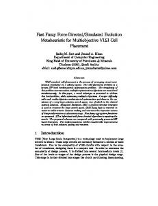
EDACE for general types of box-constrained optimisation while the latter is the real-world application. 3.1. CEC2015 Learning-Based Test Problems. The CEC2015 learning-based test problems are box-constrained single objective benchmark functions proposed in [56]. The problems consist of 2 Unimodal Functions, 3 Simple Multimodal Functions, 3 Hybrid Functions, and 7 Composition Functions. The summary of CEC2015 learning-based test problems is shown in Table 1. It should be noted that the details and the codes for the test problems can be downloaded from the website of CEC2015 competition. 3.2. Flight Dynamic Control Optimisation Problem. Flight dynamic control system design is a classical important application for real engineering problems. The motion of an aircraft can be described using the body axes which is herein the stability axes consisting of roll axis (𝑥), pitch axis (𝑦), and yaw axis (𝑧) as shown in Figure 1. The motion of the aircraft is described by Newton’s 2nd law or equations of motion for both translational and rotational motions. The dynamical model is nonlinear but can be linearised by applying aerodynamic derivatives. Due to aircraft symmetry with respect to the 𝑥𝑧 plane, the linearised dynamical model can be decoupled into two groups as longitudinal motion and the lateral/directional motion. For more details of deriving the equations of motion, see [57]. In this work, only the lateral/ directional motion control is considered. A state equation representing the dynamic motion of an aircraft is expressed as follows [57–60]: ẋ = Ax + Bu,
(5)
Mathematical Problems in Engineering
5
Table 1: Summary of CEC2015 learning-based functions. Number
Functions
𝑓min
1
Rotated high conditioned elliptic function
100
2
Rotated Cigar function
200
3
Shifted and rotated Ackley’s function
300
4
Shifted and rotated Rastrigin’s function
400
Unimodal functions
Simple multimodal functions
Hybrid functions
Composition functions
5
Shifted and rotated Schwefel’s function
500
6
Hybrid function 1 (𝑁 = 3)
600
7
Hybrid function 2 (𝑁 = 4)
700
8
Hybrid function 3 (𝑁 = 5)
800
9
Composition function 1 (𝑁 = 3)
900
10
Composition function 2 (𝑁 = 3)
1000
11
Composition function 3 (𝑁 = 5)
1100
12
Composition function 4 (𝑁 = 5)
1200
13
Composition function 5 (𝑁 = 5)
1300
14
Composition function 6 (𝑁 = 7)
1400
15
Composition function 7 (𝑁 = 10)
1500
where x = {𝛽, 𝑟, 𝑝, 𝜙}𝑇 , 𝛽 is the sideslip, a velocity in 𝑦 direction, 𝑟 is the yaw rate, rate of change of rotation about the 𝑥-axis, 𝑝 is the roll rate, rate of change of rotation about the 𝑧-axis, 𝜙 is the bank angle, rotation about the 𝑥-axis, A is the kinetic energy matrix, B is Coriolis matrix, u = { 𝛿𝛿𝑎𝑟 } is the control vector, 𝛿𝑎 is the aileron deflection, and 𝛿𝑟 is the rudder deflection. The control vector u can be expressed as u = Cu𝑝 + Kx,
𝑘6 𝑘1 𝑘2 0 K=[ ], 𝑘7 𝑘3 𝑘4 0
Roll axis Yaw axis
Figure 1: Stability axes of an aircraft.
(7) to minimise spiral root subjected to stability performance constraints. The optimisation problem can then be written as
where parameters 𝑘1 –𝑘7 are control gain coefficients which need to be found. From (5)-(6), the state equation for lateral/directional motion of an aircraft can be expressed as ẋ = (A + BK) x + BCu𝑝 .
CG
(6)
where u𝑝 is a pilot’s control input vector while C and K are the gain matrices expressed as follows [59]: 1 0 ], C=[ 𝑘5 1
Pitch axis
(8)
Design optimisation of the control system of an aircraft is found to have many objectives as there are several criteria that need to be satisfied such as control stability, accuracy, sensitivity, and control effort, while the control gains coefficients are set to be design variables for an optimisation problem. In this work, the optimal flight control of an aircraft focuses on only the stability aspect. The objective function is posed
𝜉𝐷 ≥ 0.5 𝜔𝑑 ≥ 1, where 𝜆 𝑠 , 𝜆 𝑅 , 𝜉𝐷, and 𝜔𝑑 are spiral root, roll damping, damping ratio of Dutch-roll complex pair, and Dutch-roll frequency, respectively. These parameters can be calculated based on the eigenvalues associated with the matrix A + BK. The design variables are control gain coefficients in the matrix
6
Mathematical Problems in Engineering
K (x = {𝑘1 , 𝑘2 , 𝑘3 , 𝑘4 , 𝑘6 , 𝑘7 }𝑇 ). The kinetic energy matrix (A) and the Coriolis matrix (B) are defined as −0.2842
More details about this aircraft dynamic model can be found in [58–60]. To handle the constraints, the penalty function which was presented in [61] is used. The proposed EDACE and several well-established binary-code metaheuristics are used to solve the fifteen CEC2015 learning-based test problems and the flight dynamic control test problem. The metaheuristic optimisers are as follows: Genetic algorithm (GA) [21] used binary codes with crossover and mutation rates are 1 and 0.1, respectively. Binary simulated annealing (BSA) [50] used binary codes with exponentially decreasing temperature. The starting and ending temperature are set to be 10 and 0.001, respectively. The cooling step is set as 10. Population-based incremental learning (PBIL) [24] used binary codes with the learning rate, mutation shift, and mutation rate as 0.5, 0.7, and 0.2, respectively. Binary particle swarm optimisation (BPSO) [49] used binary codes with V-shaped transfer function while the transfer function used is the V-shaped version 4 (V4) as reported in [49]. It is noted that this version is said to be the most efficient version based on the results obtained in [49]. Univariate marginal distribution algorithm (UMDA) [48] used binary codes. The first 20 best binary solutions are used to update the probability matrix. Estimation of distribution algorithm with correlation of binary elements (EDACE) (Algorithm 2) used binary codes with 𝑃𝐿 = 0.1, 𝑃𝑈 = 0.9, 𝐿 𝑅,𝐿 = 0.4, 𝐿 𝑅,𝑈 = 0.6, and 𝑛best = 10. Each algorithm is used to solve the problems for 30 optimisation runs. The population sizes are set to be 100 and 20 while number of generation is set to be 100 and 500 for the CEC2015 learning-based test problems and the flight dynamic control test problem, respectively. For an algorithm using different population size and number of generations such as BSA, it will be terminated at the same number function evaluations, which is 10,000 for all test problems. The binary length is set to be 5 for each design variable for all optimisers.
4. Optimum Results 4.1. CEC2015. After applying the proposed EDACE and several well-established binary MHs for solving the CEC2015 learning-based benchmark functions, the results are shown in Tables 2–4. Note that, apart from the algorithms used in this study, the results of solving CEC2015 test suit obtained from efficient binary artificial bee colony algorithm based on genetic operator (GBABC), binary quantum-inspired gravitational search algorithm (BQIGSA), and self-adaptive binary variant of a differential evolution algorithm (SabDE) as reported in [53] are also included in the comparison. From Table 2, the mean (Mean) and standard deviation (STD) values of the objective functions are used to measure the search convergence and consistency of the algorithms. The lower Mean is the better convergence while the lower STD is the better consistency. The value of Mean is more important; thus, for method A with lower Mean but higher STD than method B, method A is considered to be superior. For the measure of search convergence based on the mean objective function values, the best performer for the unimodal test functions, 𝑓1 and 𝑓2, is EDACE while the second best is BPSO. For the simple multimodal functions, the best performer for 𝑓4 and 𝑓5 is SabDE while the best performer for 𝑓3 is BPSO. The second best performers for 𝑓3, 𝑓4, and 𝑓5 are SabDE, BEDACE, and UMDE, respectively. For the hybrid functions, the best performers for the functions 𝑓6, 𝑓7, and 𝑓8, are SabDE, EDACE, and BPSO, respectively, while the second best performer for 𝑓6 and 𝑓7 is BPSO and the second best for 𝑓8 is EDACE. For the final group of CEC2015 test problems, composition functions, the best performer for the 𝑓11, 𝑓12, and 𝑓14 is SabDE while the best performers for the 𝑓10 and 𝑓15 are BPSO and EDACE, respectively. For 𝑓9, the best performers are UMDA, BPSO, GA, PBIL, and EDACE, which obtain the same mean values while, for 𝑓13, the best performers are UMDA, BPSO, GA, PBIL, BSA, and EDACE, which obtained the same mean values. It should be noted that the results from [53] were obtained from using the total number of function evaluations as 1,000,000 with the binary length of 50 for each design variable whereas this work uses 10,000 function evaluations with the binary length of 5 for each design variable. This indirect comparison with GBABC, BQIGSA, and SabDE can only be used to show that the proposed EDACE also has good performance and cannot be used to claim which method is superior. For the measure of search consistency based on the STD values, the most consistent methods for unimodal functions, 𝑓1 and 𝑓2, are BPSO and EDACE while the second most consistent methods are EDACE and BPSO, respectively. For the simple multimodal functions, the best for 𝑓3 and 𝑓5 is SabDE while the best for 𝑓4 is the proposed EDACE. EDACE is the best for the hybrid function of 𝑓7 while BPSO is the best for the hybrid functions 𝑓6 and 𝑓8. For the composition functions, EDACE is the best for the problems 𝑓9 and 𝑓12 while BPSO is the best for 𝑓10. For the composition functions, 𝑓11, 𝑓14, and 𝑓15, the best is SabDE while the best for 𝑓13 is BSA.
∗
𝑓15
𝑓14
𝑓13
𝑓12
𝑓11
𝑓10
𝑓9
𝑓8
𝑓7
𝑓6
𝑓5
𝑓4
𝑓3
𝑓2
𝑓1
MHs Mean STD Min. Mean STD Min Mean STD Min Mean STD Min Mean STD Min Mean STD Min Mean STD Min Mean STD Min Mean STD Min Mean STD Min Mean STD Min Mean STD Min Mean STD Min Mean STD Min Mean STD Min
Mathematical Problems in Engineering Table 3: Ranking of all optimisers based on the Mean values. UMDA 4 4 9 3 2 4 5 4 3 3 9 4 3 9 6 72
𝑓1 𝑓2 𝑓3 𝑓4 𝑓5 𝑓6 𝑓7 𝑓8 𝑓9 𝑓10 𝑓11 𝑓12 𝑓13 𝑓14 𝑓15 Sum of ranking
BPSO 2 2 1 4 4 2 2 1 2 1 4 6 2 4 3 40
GA 3 5 8 7 7 5 3 3 5 4 6 7 6 6 5 80
PBIL 5 3 7 6 8 6 4 5 4 5 7 9 5 7 4 85
BSA 7 6 4 5 6 8 6 6 6 7 8 8 1 8 7 93
EDACE 1 1 3 2 3 3 1 2 1 2 5 5 4 5 2 40
GBABC 6 8 5 8 5 9 8 9 7 8 2 3 7 2 9 96
BQIGSA 8 9 5 9 9 7 7 7 8 6 3 2 8 3 1 92
SabDE 9 7 2 1 1 1 9 8 9 9 1 1 9 1 8 76
BQIGSA 0
SabDE 0
Table 4: Comparison based on the statistical 𝑡-test of the test problem. UMDA 0
BPSO 1
BPSO
0
0
0
0
0
1
0
0
0
GA
0
1
0
0
0
1
0
0
0
PBIL
1
1
1
0
0
1
0
0
0
BSA
1
1
1
1
0
1
1
0
0
EDACE
0
0
0
0
0
0
0
0
0
GBABC
1
1
1
1
0
1
0
0
0
BQIGSA
1
1
1
1
1
1
1
0
0
UMDA
GA 1
PBIL 0
BSA 0
EDACE 1
GBABC 0
SabDE
1
1
1
1
1
1
1
1
0
Sum
5
7
6
4
2
8
3
1
0
Ranking
4
2
3
5
7
1
6
8
9
The value Min in Table 2 is the objective function value of the best run from a particular method. Note that only the UMDA, BPSO, GA, PBIL, BSA, and EDACE were compared. For the unimodal function, the minimum objective function values of 𝑓1 and 𝑓2 were obtained by BPSO and EDACE, respectively. For the simple multimodal functions, the minimum objective function values for 𝑓3 and 𝑓5 are obtained from BPSO and EDACE, respectively, while for 𝑓4, the minimum is obtained from UMDA, BSA, and EDACE. The EDACE obtained minimum objective function values for all test functions in the hybrid function group. However, for the hybrid function 𝑓8, three algorithms including BPSO, GA, and EDACE obtained the minimum values. For the composition functions, EDACE obtained the minimum function values for all test functions. However, for the functions 𝑓9 and 𝑓13, all algorithms obtained the same minimum values while
for the 𝑓11, BPSO and EDACE obtained the same minimum function values. Similarly, for 𝑓12, UMDA, BPSO, BSA, and EDACE obtained the same minimum values. Table 3 shows the summary of ranking based on the mean objective function values from 30 optimisation runs. It was found that the proposed EDACE is mostly ranked in top three best from solving fifteen CEC2015 learning-based test problems. After summing up the ranking score, it is found that EDACE and BPSO are equal best performer while the third best is UMDA. In order to further investigate the performance comparison of the binary-code MHs, the statistical 𝑡-test is employed. Table 4 shows a 9 × 9 comparison matrix of the 9 optimisers. If method 𝑖 is significantly better than method 𝑗 based on the 𝑡-test at 5% significant level, the column 𝑖 and row 𝑗 of the matrix are set to be 1; otherwise, they are set to be 0. When
Mathematical Problems in Engineering ×108 4
9 ×10⁹ 18
f1
16
3.5
14
2.5
Obj. function value
Obj. function value
3
2 1.5 1
12 10 8 6 4
0.5 0
f2
2 0
1
2
3 4 5 6 7 8 Number of ffunction evaluations
9
0
10 ×104
0
1
2
3
4
5
6
7
8
Number of function evaluations
9
10 ×104
UMDA BPSO BEDACE
UMDA BPSO BEDACE
Figure 2: Search history of the top three best optimisers based on the 𝑡-test for the unimodal function.
Table 5: Ranking of all optimisers for all CEC2015 learning-based test problem based on statistical 𝑡-test. 𝑓1 𝑓2 𝑓3 𝑓4 𝑓5 𝑓6 𝑓7 𝑓8 𝑓9 𝑓10 𝑓11 𝑓12 𝑓13 𝑓14 𝑓15 Sum
UMDA 4 4 5 3 2 4 3 4 3 3 9 4 1 9 6 64
BPSO 2 2 2 4 4 2 1 1 1 1 4 5 1 4 3 37
GA 3 5 5 6 7 5 3 3 4 4 6 7 1 6 5 70
PBIL 5 3 5 6 8 6 3 5 4 5 7 8 1 7 4 77
summing up along the columns, the highest score indicates the best optimiser based on this type of comparison. In the table, it means EDACE is the best. Table 5 shows the ranking of the 9 optimisers when solving all CEC2015 learning-based test problems based on the 𝑡-test. After summing up the ranking numbers of all test problems, it is found that EDACE is the overall best optimiser while BPSO and UMDA are the second and the third best, respectively.
BSA 7 6 4 4 6 8 6 6 6 7 8 8 1 8 7 92
EDACE 1 1 2 2 2 3 1 2 1 2 5 5 1 5 2 35
GBABC 6 8 5 8 5 9 8 9 7 8 2 2 7 2 9 95
BQIGSA 8 9 5 8 9 7 7 7 8 6 2 2 7 3 1 89
SabDE 9 7 1 1 1 1 8 8 9 9 1 1 9 1 8 74
Figures 2–5 show the search history of the top three optimisers EDACE, BPSO, and UMDA on solving all CEC2015 learning-based test problems where the vertical axis is the average objective function from 30 runs of each method. For all test functions, it was found that EDACE and UMDA converged to the optimal values at higher speed while BPSO seems to converge slowly and consistently. However, for all functions, BPSO finally moves to the minimum or near
10
Mathematical Problems in Engineering f3
320.8
520
320.6
500
320.4 320.2 320 319.8 319.6
f4
540
Obj. function value
Obj. function value
321
480 460 440 420
0
1
2
3
4
5
6
7
8
Number of function evaluations
9
10 ×104
400
0
1
2
3 4 5 6 7 8 Number of function evaluations
9
10 ×104
UMDA BPSO BEDACE
UMDA BPSO BEDACE f5
3500
Obj. function value
3000 2500 2000 1500 1000
0
1
2
3 4 5 6 7 8 Number of function evaluations
9
10 ×104
UMDA BPSO BEDACE
Figure 3: Search history of the top three best optimisers based on the 𝑡-test for the simple multimodal functions.
Table 6: The table shows performance of EDACE for various number of binary bits. Number of binary bits Mean function values Average computational time (Sec.)
5 2.314𝐸 + 6 9.371
minimum function values at the end of the runs. EDACE shows fast convergence from the beginning and obtained the minimum or near minimum values for all test functions except for 𝑓3. This indicates the ability of search exploitation and search exploration of the proposed EDACE since the CEC2015 test functions were assigned to test both aspects of MHs. Table 6 shows performance of EDACE on solving unimodal function, 𝑓1, when the binary lengths for each design variable are 5, 10, 25, and 50 for 10 optimisation runs. It was found that when the number of binary bits increases, the computational time increases and the resulting mean objective function values decrease for the binary lengths less
10 1.101𝐸 + 6 10.748
25 1.079𝐸 + 6 18.634
50 1.143𝐸 + 6 52.773
than 25. However, for the binary length of 50, the mean objective function value increases meaning EDACE performance deteriorates. Without considering computational time, the best number of binary length is 25. 4.2. Flight Dynamic Control System Design. After applying the six binary-code MHs to solve the real engineering application of flight dynamic and control system for 30 optimisation runs, the comparison results are shown as box-plots of the objective and constraint violation values (Figure 6). The upper and lower horizontal lines of each box represent the maximum and minimum of objective function values, respectively, while the internal line shows the median
Mathematical Problems in Engineering ×107 3
11
f6
760 Obj. function value
Obj. function value
2.5 2 1.5 1 0.5 0
f7
770
750 740 730 720 710
0
1
2
3 4 5 6 7 8 Number of function evaluations
9
10 ×104
700
0
1
2
3 4 5 6 7 8 Number of function evaluations
9
10 ×104
UMDA BPSO BEDACE
UMDA BPSO BEDACE ×106 4.5
f8
Obj. function value
4 3.5 3 2.5 2 1.5 1 0.5 0
0
1
2
3 4 5 6 7 8 Number of function evaluations
9
10 ×104
UMDA BPSO BEDACE
Figure 4: Search history of the top three best optimisers based on the 𝑡-test for the hybrid functions.
of objective function values. From this figure, based on median values of objective function, it is found that the best performer is EDACE while the second best and the third best are BPSO and UMDA, respectively. The most consistent method having the smallest gap between the maximum and minimum for all of optimisation runs is UMDA. However, the worst function value found by EDACE is almost as good as the best found by UMDA. Thus, the proposed EDACE is superior. Based on the figure, it was found that GA failed to solve the problem as it cannot obtain a feasible optimum point. The minimum objective function value is obtained from using the proposed EDACE. Figure 7 shows the best run search history of all optimisers (selection based on the minimum objective function values of feasible solutions). From the figure, UMDA and PBIL seem to be the fastest convergent methods initially. However, after the process goes on for about 4,000 function evaluations, the proposed EDACE converged to the minimum objective function value with a faster rate than the others. It has better
exploration rate as the best function value is still decreased at the late iteration numbers. BPSO, on the other hand, seems to be slower than UMDA, PBIL, and BSA in the beginning. It however can converge to the better results after around 8,000 function evaluations.
5. Conclusions and Discussion In this work, a new concept of a binary-code optimiser is proposed. Fifteen CEC2015 learning-based test problems and a real engineering design problem of flight dynamic and control system are used to investigate the search performance of the proposed algorithm. Several well-established binarycode MHs are used in comparison. The results obtained show that the proposed EDACE is the best performer on solving the 15 CEC2015 learning-based test problems and real engineering design problem of flight dynamic and control. Further improvement of EDACE by means of self-adaptation will be investigated in the future. The choice for bREF needs further
Mathematical Problems in Engineering ×106 6
f9
1100
Obj. function value
Obj. function value
12
1050 1000
0
1
2
3 4 5 6 7 8 Number of function evaluations
9
10
4 2 0
0
Obj. function value
Obj. function value
f11
1600 1400 1
2
3 4 5 6 7 8 Number of function evaluations
9
10 ×104
1340 1320 2
10 ×104
f12
1350 1300
Obj. function value
Obj. function value
f13
1
9
0
1
2
3 4 5 6 7 8 Number of function evaluations
9
10 ×104
UMDA BPSO BEDACE
1360
0
3 4 5 6 7 8 Number of function evaluations
1400
UMDA BPSO BEDACE
1300
2
UMDA BPSO BEDACE
1800
0
1
×104
UMDA BPSO BEDACE
1200
f10
3
4
5
6
7
8
9
10
×104 3
f14
2 1 0
0
1
2
×104
Number of function evaluations
9
10 ×104
UMDA BPSO BEDACE Obj. function value
UMDA BPSO BEDACE
3 4 5 6 7 8 Number of function evaluations
10000
f15
5000 0
0
1
2
3 4 5 6 7 8 Number of function evaluations
9
10 ×104
UMDA BPSO BEDACE
Figure 5: Search history of the top three best optimisers based on the 𝑡-test for the composition functions.
studies. The use of EDACE for hyperheuristic development is also possible. The extension to multiobjective optimisation and many-objective optimisation is also under investigation. Appling EDACE for the more complex problems such as large scale problems, mixed-variable problems, and reliability optimisation is for future work. The fight control optimisation problem, one of our recent research focuses, has more than three objective functions to be optimised; thus, it should be formulated as many-objective optimisation. This along
with aircraft path planning dynamic optimisation still needs considerably more investigation while EDACE will be one of optimisers to be used for solving such design problems.
Conflicts of Interest The authors declare that there are no conflicts of interest regarding the publication of this article.
Objective function values
Mathematical Problems in Engineering
13
−0.1 −0.2
Maximum constraints values
−0.3 BPSO
GA
PBIL BSA Algorithms
UMDA
EDACE
BPSO
GA
PBIL BSA Algorithms
UMDA EDACE
400 200 0
Figure 6: Box-plot of objective function values from 30 optimisation runs. 0.2
Objective function values
0.1 0 −0.1 −0.2 −0.3 −0.4
0
1000 2000 3000 4000 5000 6000 7000 8000 9000 10000 Number of function evaluations BPSO GA PBIL
BSA UMDA EDACE
Figure 7: Search history of the best run of all optimisers.
Acknowledgments The authors are grateful for the support from the Thailand Research Fund (TRF), Grant no. MRG5980238.
References [1] S. Mirjalili, “Moth-flame optimization algorithm: a novel nature-inspired heuristic paradigm,” Knowledge-Based Systems, vol. 89, pp. 228–249, 2015. [2] R. V. Rao, V. J. Savsani, and D. P. Vakharia, “Teaching-learningbased optimization: a novel method for constrained mechanical design optimization problems,” Computer-Aided Design, vol. 43, no. 3, pp. 303–315, 2011. [3] Y. Tan and Y. Zhu, “Fireworks algorithm for optimization,” in Advances in Swarm Intelligence, Y. Tan, Y. Shi, and K. Tan, Eds., vol. 6145, pp. 355–364, Springer, Berlin Heidelberg, Germany, 2010.
[4] A. Kaveh and S. Talatahari, “A novel heuristic optimization method: charged system search,” Acta Mechanica, vol. 213, no. 3-4, pp. 267–289, 2010. [5] E. Rashedi, H. Nezamabadi-pour, and S. Saryazdi, “GSA: a gravitational search algorithm,” Information Sciences, vol. 179, no. 13, pp. 2232–2248, 2009. [6] M. Fesanghary, “Harmony search applications in mechanical, chemical and electrical engineering,” in Music-Inspired Harmony Search Algorithm, Z. Geem, Ed., vol. 191, pp. 71–86, Springer Publishing Company, Berlin, Heidelberg, Germany, 2009. [7] X. Wu, Y. Zhou, and Y. Lu, “Elite opposition-based water wave optimization algorithm for global optimization,” Mathematical Problems in Engineering, vol. 2017, Article ID 3498363, 25 pages, 2017. [8] C. Wang, Y. Wang, K. Wang, Y. Dong, and Y. Yang, “An improved hybrid algorithm based on biogeography/complex and Metropolis for many-objective optimization,” Mathematical Problems in Engineering, vol. 2017, Article ID 2462891, 14 pages, 2017.
14 [9] W. Lei, H. Manier, M.-A. Manier, and X. Wang, “A hybrid quantum evolutionary algorithm with improved decoding scheme for a robotic flow shop scheduling problem,” Mathematical Problems in Engineering, vol. 2017, Article ID 3064724, 13 pages, 2017. [10] C.-R. Hwang, “Simulated annealing: theory and applications,” Acta Applicandae Mathematicae, vol. 12, pp. 108–111, 1988. [11] C. Qu, S. Zhao, Y. Fu, and W. He, “Chicken swarm optimization based on elite opposition-based learning,” Mathematical Problems in Engineering, vol. 2017, Article ID 2734362, 20 pages, 2017. [12] N. Dong, X. Fang, and A.-g. Wu, “A novel chaotic particle swarm optimization algorithm for parking space guidance,” Mathematical Problems in Engineering, vol. 2016, Article ID 5126808, 14 pages, 2016. [13] X.-S. Yang and A. H. Gandomi, “Bat algorithm: a novel approach for global engineering optimization,” Engineering Computations, vol. 29, no. 5, pp. 464–483, 2012. [14] X.-S. Yang and S. Deb, “Engineering optimisation by Cuckoo search,” International Journal of Mathematical Modelling and Numerical Optimisation, vol. 1, no. 4, pp. 330–343, 2010. [15] K. Socha and M. Dorigo, “Ant colony optimization for continuous domains,” European Journal of Operational Research, vol. 185, no. 3, pp. 1155–1173, 2008. [16] D. Karaboga and B. Basturk, “A powerful and efficient algorithm for numerical function optimization: artificial bee colony (ABC) algorithm,” Journal of Global Optimization, vol. 39, no. 3, pp. 459–471, 2007. [17] G. Venter and J. Sobieszczanski-Sobieski, “Particle swarm optimization,” AIAA Journal, vol. 41, no. 8, pp. 1583–1589, 2003. [18] V. Muthiah-Nakarajan and M. M. Noel, “Galactic swarm optimization: a new global optimization metaheuristic inspired by galactic motion,” Applied Soft Computing Journal, vol. 38, pp. 771–787, 2016. [19] S. Mirjalili and A. Lewis, “The whale optimization algorithm,” Advances in Engineering Software, vol. 95, pp. 51–67, 2016. [20] S. Mirjalili, S. M. Mirjalili, and A. Lewis, “Grey wolf optimizer,” Advances in Engineering Software, vol. 69, pp. 46–61, 2014. [21] D. E. Goldberg and J. H. Holland, “Genetic algorithms and machine learning,” Machine Learning, vol. 3, no. 2-3, pp. 95–99, 1998. [22] R. Storn and K. Price, “Differential evolution—a simple and efficient heuristic for global optimization over continuous spaces,” Journal of Global Optimization, vol. 11, no. 4, pp. 341– 359, 1997. [23] T. B¨ack, Evolutionary Algorithms in Theory and Practice, Oxford University Press, New York, NY, USA, 1996. [24] S. Baluja, Population-Based Incremental Learning: A Method for Integrating Genetic Search Based Function Optimization and Competitive Learning, Carnagie Mellon University, Pittsburgh, PA, USA, 1994. [25] L. J. Fogel, A. J. Owens, and M. J. Walsh, Artificial Intelligence through Simulated Evolution, John Wiley, New York, NY, USA, 1966. [26] H. Beyer and H. Schwefel, “Evolution strategies—a comprehensive introduction,” Natural Computing, vol. 1, no. 1, pp. 3–52, 2002. [27] S. Mirjalili, “SCA: a sine cosine algorithm for solving optimization problems,” Knowledge-Based Systems, vol. 96, pp. 120–133, 2016. [28] R. V. Rao, “Jaya: a simple and new optimization algorithm for solving constrained and unconstrained optimization problems,” International Journal of Industrial Engineering Computations, vol. 7, no. 1, pp. 19–34, 2016.
Mathematical Problems in Engineering [29] J. Q. Zhang and A. C. Sanderson, “JADE: adaptive differential evolution with optional external archive,” IEEE Transactions on Evolutionary Computation, vol. 13, no. 5, pp. 945–958, 2009. [30] R. Tanabe and A. Fukunaga, “Evaluating the performance of SHADE on CEC 2013 benchmark problems,” in Proceedings of the 2013 IEEE Congress on Evolutionary Computation (CEC ’13), pp. 1952–1959, June 2013. [31] R. Tanabe and A. S. Fukunaga, “Improving the search performance of shade using linear population size reduction,” in Proceedings of the IEEE Congress on Evolutionary Computation (CEC ’14), pp. 1658–1665, IEEE, July 2014. [32] M. P. Wachowiak, M. C. Timson, and D. J. DuVal, “Adaptive particle swarm optimization with heterogeneous multicore parallelism and GPU acceleration,” IEEE Transactions on Parallel and Distributed Systems, 2017. [33] L. Zhang, Y. Tang, C. Hua, and X. Guan, “A new particle swarm optimization algorithm with adaptive inertia weight based on Bayesian techniques,” Applied Soft Computing Journal, vol. 28, pp. 138–149, 2015. [34] X. Liang, W. Li, Y. Zhang, and M. C. Zhou, “An adaptive particle swarm optimization method based on clustering,” Soft Computing, vol. 19, no. 2, pp. 431–448, 2015. [35] N. Srinivas and K. Deb, “Multiobjective function optimization using nondominated sorting genetic algorithms,” Evolutionary Computation, vol. 2, pp. 221–248, 1994. [36] K. Deb, A. Pratap, S. Agarwal, and T. Meyarivan, “A fast and elitist multiobjective genetic algorithm: NSGA-II,” IEEE Transactions on Evolutionary Computation, vol. 6, no. 2, pp. 182– 197, 2002. ´ [37] W. Mkaouer, M. Kessentini, S. Bechikh, K. Deb, and M. O. Cinn´eide, “High dimensional search-based software engineering: Finding tradeoffs among 15 objectives for automating software refactoring using NSGA-III,” in Proceedings of the 16th Genetic and Evolutionary Computation Conference (GECCO ’14), pp. 1263–1270, July 2014. [38] C. A. Coello Coello and M. S. Lechuga, “MOPSO: a proposal for multiple objective particle swarm optimization,” in Proceedings of the Congress on Evolutionary Computation (CEC ’02), pp. 1051–1056, May 2002. [39] E. Zitzler, M. Laumanns, and L. Thiele, “SPEA2: improving the strength Pareto evolutionary algorithm for multiobjective optimization, presented at the Evolutionary Methods for Design, Optomozation and Control,” Evolutionary Methods for Design, Optomozation and Control, Barcelona Spain, 2002. [40] K. Nuaekaew, P. Artrit, N. Pholdee, and S. Bureerat, “Optimal reactive power dispatch problem using a two-archive multiobjective grey wolf optimizer,” Expert Systems with Applications, vol. 87, pp. 79–89, 2017. [41] F. Zou, L. Wang, X. Hei, D. Chen, and B. Wang, “Multi-objective optimization using teaching-learning-based optimization algorithm,” Engineering Applications of Artificial Intelligence, vol. 26, no. 4, pp. 1291–1300, 2013. [42] Q. Zhang and H. Li, “MOEA/D: a multiobjective evolutionary algorithm based on decomposition,” IEEE Transactions on Evolutionary Computation, vol. 11, no. 6, pp. 712–731, 2007. [43] D. Angus and C. Woodward, “Multiple objective ant colony optimisation,” Swarm Intelligence, vol. 3, no. 1, pp. 69–85, 2009. [44] B. V. Babu and M. M. L. Jehan, “Differential evolution for multi-objective optimization,” in Proceedings of the Congress on Evolutionary Computation (CEC ’03), pp. 2696–2703, Canberra, Australia, December 2003. [45] X. Zhang, Y. Tian, and Y. Jin, “A knee point driven evolutionary algorithm for many-objective optimization,” IEEE Transactions on Evolutionary Computation, vol. 19, no. 6, pp. 761–776, 2015.
Mathematical Problems in Engineering [46] H. Wang, L. Jiao, and X. Yao, “Two Arch2: an improved twoarchive algorithm for many-objective optimization,” IEEE Transactions on Evolutionary Computation, vol. 19, no. 4, pp. 524–541, 2015. [47] R. Wang, R. C. Purshouse, and P. J. Fleming, “Preferenceinspired coevolutionary algorithms for many-objective optimization,” IEEE Transactions on Evolutionary Computation, vol. 17, no. 4, pp. 474–494, 2013. [48] H. M¨uhlenbein, “The equation for response to selection and its use for prediction,” Evolutionary Computation, vol. 5, no. 3, pp. 303–346, 1997. [49] S. Mirjalili and A. Lewis, “S-shaped versus V-shaped transfer functions for binary particle swarm optimization,” Swarm and Evolutionary Computation, vol. 9, pp. 1–14, 2013. [50] S. Bureerat and J. Limtragool, “Structural topology optimisation using simulated annealing with multiresolution design variables,” Finite Elements in Analysis and Design, vol. 44, no. 12-13, pp. 738–747, 2008. [51] C. Ozturk, E. Hancer, and D. Karaboga, “A novel binary artificial bee colony algorithm based on genetic operators,” Information Sciences, vol. 297, pp. 154–170, 2015. [52] H. Nezamabadi-Pour, “A quantum-inspired gravitational search algorithm for binary encoded optimization problems,” Engineering Applications of Artificial Intelligence, vol. 40, pp. 62–75, 2015. [53] A. Banitalebi, M. I. A. Aziz, and Z. A. Aziz, “A self-adaptive binary differential evolution algorithm for large scale binary optimization problems,” Information Sciences, vol. 367-368, pp. 487–511, 2016. [54] B. Crawford, R. Soto, G. Astorga, J. Garcia, C. Castro, and F. Paredes, “Putting continuous metaheuristics to work in binary search spaces,” Complexity, vol. 2017, Article ID 8404231, 19 pages, 2017. [55] G. Lindfield and J. Penny, Numerical Methods: Using MATLAB, Academic Press, 2012. [56] J. Liang, B. Qu, P. Suganthan, and Q. Chen, “Problem definitions and evaluation criteria for the CEC 2015 competition on learning-based real-parameter single objective optimization,” Tech. Rep., Computational Intelligence Laboratory, Zhengzhou University, Zhengzhou China and Technical Report, Nanyang Technological University, Singapore, 2014. [57] D. A. Caughey, Introduction to Aircraft Stability and Control Course Notes for M&AE 5070, Sibley School of Mechanical & Aerospace Engineering, Cornell University, Ithaca, New York, NY, USA, 2011. [58] S. Rostami and F. Neri, “Covariance matrix adaptation pareto archived evolution strategy with hypervolume-sorted adaptive grid algorithm,” Integrated Computer-Aided Engineering, vol. 23, no. 4, pp. 313–329, 2016. [59] S. F. Adra, A. I. Hamody, I. Griffin, and P. J. Fleming, “A hybrid multi-objective evolutionary algorithm using an inverse Neural Network for aircraft control system design,” in Proceedings of the 2005 IEEE Congress on Evolutionary Computation (IEEE CEC ’05), pp. 1–8, September 2005. [60] D. Tabak, A. A. Schy, D. P. Giesy, and K. G. Johnson, “Application of multiobjective optimization in aircraft control systems design,” Automatica, vol. 15, no. 5, pp. 595–600, 1979. [61] S. Bureerat and N. Pholdee, “Optimal truss sizing using an adaptive differential evolution algorithm,” Journal of Computing in Civil Engineering, vol. 30, no. 2, p. 04015019, 2015.
15
Advances in
Operations Research Hindawi Publishing Corporation http://www.hindawi.com