set and the likelihood of feasible color mappings in respect to their fre- quency and .... â©(H1, H2) = â k min{H1(k), H2(k)} â [0, 1]. (6) .... viewed under 11 illuminants. 1 http://www.cs.sfu.ca/~color/data/objects under different lights/index. html ...
A New Color Constancy Algorithm Based on the Histogram of Feasible Mappings� Jaume Verg´es–Llah´ı and Alberto Sanfeliu Institut de Rob` otica i Inform` atica Industrial, Technological Park of Barcelona, U Building {jverges, asanfeliu}@iri.upc.edu
Abstract. Color is an important cue both in machine vision and image processing applications, despite its dependence upon illumination changes. We propose a color constancy algorithm that estimates both the set and the likelihood of feasible color mappings in respect to their frequency and effectiveness. The best among this set is selected to rendered back image colors as seen under a canonical light. Experiments were done to evaluate its performance compared to Finlayson’s 2D gamut–mapping algorithm, outperforming it. Our approach is a helpful alternative wherever illumination is poorly known since it employs only image data. Keywords: Color, color mappings, color constancy, color histograms.
1
Introduction
In a number of applications from machine vision to multimedia or even mobile robotics, it is important that the recorded colors remain constant under changes in the scene illumination. Hence, a preliminary step when using color must be to remove the distracting effects of such a variation. This problem is usually referred to as color constancy, i.e., the stability of surface color appearance under varying illumination. Part of the difficulty is its entanglement with other confounding phenomena such as object shape, viewing and illumination geometry, besides changes in the nature of light and the reflectance properties of surfaces. Generally, color constancy (CC) is understood as the recovery of descriptors for the surfaces in a scene as they would be seen under a canonical illuminant. This is similar to recover an estimate of the illumination color from an image under an unknown light, since it is relatively straightforward to map image colors back to illuminant independent descriptors [1]. Therefore, finding a mapping between colors or the color of the scene illuminant are equivalent problems. Some algorithms followed such a path, specially those related to the gamut– mapping approach [2,3,4,5]. Recently, the trend has slightly changed to make a guess on the illumination, as in color–by–correlation [1] or color–voting [6], rather than attempting to recover only one estimate. A measure of the likelihood that each of a set of feasible candidates was the scene illuminant is set out instead, which is afterwards used to render the image back into the canonical illuminant. �
Sup. by the Spanish Min. of Edu. & Sci. under proj. TIC2003-09291 & DPI2004-5414.
M. Kamel and A. Campilho (Eds.): ICIAR 2005, LNCS 3656, pp. 720–728, 2005. c Springer-Verlag Berlin Heidelberg 2005 �
A New Color Constancy Algorithm
721
Some difficulties arise among the approaches above. The main one for us is the dependence on the fact that all possible colors under a canonic illuminant be available a priori. Besides, while gamut–mapping employs a selection strategy blind to any information about the likelihood of a particular mapping, color–by– correlation can only chose an illumination out of a discrete set of lights known a priori. Real–world applications usually do not fit such requirements. Hence, in this paper we propose a new color constancy algorithm that can be used in tasks with little knowledge on the scene illumination. Our algorithm computes the histogram of the feasible maps and recovers one to changes image colors as if seen under a canonic light only using a canonic image picturing a similar scene. The performance of this algorithm is compared to that of the Finlayson’s 2D gamut–mapping, outperforming it and obtaining similar figures to those of the color–by–correlation approach.
2
The Color Constancy Algorithm
The goal of this algorithm is to recover an image as seen under some canonic illumination. This algorithm gives to each feasible color mapping a particular likelihood related to its frequency and performance. The frequency is estimated from the histogram of feasible mappings, while the performance evaluates how close colors are rendered to those in the canonic set. The combined measure is used afterwards to select the best color mapping. Hereafter, we describe the basis of our algorithm along with its elements, namely, likelihood function, color coordinates, color change model, and mapping estimation and selection. Let Ic and Ia be the canonic and the actual images, respectively, picturing similar scenes under two different lights. The algorithm only employs image raw data and no segmentation is needed. Our aim is to find the likeliest color transformation T mapping colors of image Ia as close to those of Ic as possible. We note as I ⊂ Rd a set of colors, where d is the color space dimension. Its origin can be either a specified color gamut or an image. The color histogram of I is noted as HI . If a mapping T ∈ is applied to each color in I, a transformed set T(I) is obtained. < T > is the set of feasible color mappings. Analogously, T(HI ) represents the transformation of the histogram HI by the map T. In general, given two color sets, Ia and Ic , a model of color change consists in a mapping T ∈ so that T : Ia −→ Ic s �−→ T(s) = q
(1)
where s ∈ S and q ∈ Q are corresponding colors. The set of feasible maps is = {T = ∆(S, Q) | ∀S ⊂ Ia and ∀Q ⊂ Ic } and ∆ is a mapping estimation scheme computing a map T out of two corresponding sets S and Q. 2.1
Likelihood Function
ˆ from The color constancy algorithm must select the likeliest transformation T the set accordingly to a likelihood function L∆ (T | Ia , Ic ) as
722
J. Verg´es–Llah´ı and A. Sanfeliu
ˆ = argmax { L∆ (T | Ia , Ic )} T T ∈
(2)
Any likelihood L∆ is related to a probability function Pr as L∆ (T | Ia , Ic ) = log(Pr(T | Ia , Ic )), noting that the map maximizing L∆ (T | Ia , Ic ) also maximizes Pr(T | Ia , Ic )), and vice versa. Hence, we must first get a value for the probability of any mapping T. As an estimate of Pr(T | Ia , Ic ) we use the histogram of the set of feasible mappings, noted as H . In order to compute frequencies we employ colors in the sets Ia and Ic , as well as the mapping estimator ∆. The point is that the likelier a mapping is, the more frequent it should be in the histogram H , and the other way round. Nonetheless, a particular mapping T can be produced from different groups of colors. Thus, it is useful to define the set of all pairs (S, Q) giving rise to a certain map T from the estimator ∆, i.e., ∆−1 (T) = {(S, Q) ∈ 2Ia ×2Ic | ∆(S, Q) = T}, where 2I stands for the set of all subsets of I. Therefore, the set ∆−1 (T) is equivalent to T and can be taken instead of it since ∆−1 (T) = ∆−1 (T� ) ⇔ T = T� . Hence, it is true that Pr(T | Ia , Ic ) = Pr(∆−1 (T) | Ia , Ic ). In practice, ∆−1 (T) can be thought as a finite disjoint union of singletons {(S, Q)}, being each set a combination of colors from sets Ia and Ic , respectively. Besides, to compute Pr((S, Q) | Ia , Ic ) we must only remind that each {(S, Q)} is formed by two independent sets, namely, S ⊂ Ia and Q ⊂ Ic . Therefore, Pr((S, Q) | Ia , Ic ) = Pr(S | Ia ) · Pr(Q | Ic )
(3)
Then, we get that �
Pr(T | Ia , Ic )) =
Pr(S | Ia ) · Pr(Q | Ic )
(4)
∀(S,Q)∈∆−1 (T)
that is, frequency of a mapping T in the histogram of feasible mappings H is computed adding the product of frequencies corresponding to all the pairs S and Q giving rise to the mapping T by means of the mapping estimator ∆. Pr(S | Ia ) and Pr(Q | Ic ) are approximated by the frequency of the corresponding bins in histograms HIa and HIc . In case S = {s}, it is straightforward that Pr(S | I) ≈ HI (s). Hence, in general, if S = {si }i=1,...,n , the probability of the set under the hypothesis of independence of colors is n � HI (si ) (5) Pr(S | I) ≈ i=1
On the other hand, usually some spurious peaks appear in H , which might mislead the algorithm. To improve the robustness of Eq. (4), a measure of similarity between the transformed set T(Ia ) and the canonic set Ic is taken into account, evaluating the efficiency of a particular mapping T. We use the Swain & Ballard intersection–measure between histograms defined in [7] as � min{H1 (k), H2 (k)} ∈ [0, 1] (6) ∩(H1 , H2 ) = k
A New Color Constancy Algorithm
723
The advantages of such a measure are that it is very fast to compute if compared to other matching functions. Besides, if the histograms are sparse and colors equally probable, it is a robust way of comparing images [7]. This step helps in practice to eliminate outlier mappings among candidates. As a consequence, we finally define our likelihood function by joining the probability of a mapping and its performance in a single expression as follows L∆ (T | Ia , Ic ) = log(∩(T(HIa ), HIc )) · Pr(T | Ia , Ic )) , ∀T ∈
(7)
where T(HIa ) is the transformation of HIa by a mapping T and Pr(T | Ia , Ic )) is the frequency of T in the histogram H computed with Eq. (4). 2.2
Color Coordinates
Colors can be represented as vectors in Rd . In our case, to alleviate problems with specularities or shape and to reduce at the same time the computational burden, we use the perspective color coordinates (r, g) = (R/B, G/B) proposed by Finlayson in [3]. Finlayson and Hordley also proved in [8] for these coordinates that the set of feasible mappings computed in a 3D space and projected into a 2D space afterward is the same as the one directly computed in a 2D space. 2.3
Color Change Model
It is been stated that any color change could be described using a homogeneous linear relation [2]. Thus, the mapping T is specified in coordinates as follows T : Ia −→ Ic s �−→ T(s) = T st = qt
(8)
A reasonable tradeoff between simplicity and performance is attained employing a diagonal model [2,1,3]. This model assumes color sensors are completely uncorrelated and any change in the light falling into them equates to independently scaling each channel, that is, T = diag(t1 , . . . , td ). Equivalently, T can be expressed as a vector t = (t1 , . . . , td ) ∈ Rd , so that, T = t Id . This is the model used in this paper, despite the color constancy algorithm also works with any other more complete model, involving more computational time as a result. 2.4
Mapping Estimation
Formally, the mapping estimator ∆ is a function computing a mapping T ∈ from two sets S = {si }i=1,...,n ⊂ Ia and Q = {qi }i=1,...,n ⊂ Ic , i.e., ∆ : 2Ia × 2Ic −→ (S, Q) �−→ ∆(S, Q) = T
(9)
A mapping T can be expressed as a matrix T so that q = T(s) is equivalent to T st = qt . In general, it is not possible to find a matrix T out of just a
724
J. Verg´es–Llah´ı and A. Sanfeliu
pair of corresponding vectors s and q, since we need, at least, as many linearly independent pairs as the space dimension d. Taking advantage of the nature of T and two sets of n ≥ d one–to–one corresponding vectors, namely, {si }i=1,...,n and {qi }i=1,...,n , it is true that T (st1 | · · · | stn ) = (qt1 | · · · | qtn ). If S = (st1 | · · · | stn ) ∈ Md×n (R) and Q = (qt1 | · · · | qtn ) ∈ Md×n (R) are introduced by joining vectors columnwise, finding a matrix T consists in solving the linear system Q = T S, where T is the unknown. The usual method to solve this system is by a SVD to compute pseudo–inverse S+ . Therefore, the version of Eq. (9) in coordinates is ∆ : Md×n (R) × Md×n (R) −→ Md (R) (S, Q) �−→ ∆(S, Q) = Q S+ = T
(10)
In case the diagonal model is used, the above function is greatly simplified ∆ : Rd × Rd −→ Rd (s, q) �−→ ∆(s, q) = ( qs11 , . . . , sqdd )t = t
(11)
The method for carrying out the mapping computations between two color sets consists in first computing the histograms of both sets and applying the estimator ∆ to every possible pair of color sets. Colors in S need not to be really in a correspondence with those in Q, since all possible combinations are checked. Nevertheless, in a real case some heuristic are necessary to speed up the process. In our case, only the colors with nonzero frequency � � are considered, which reduces the amount of computations to less than O p2 , where p n is the number of histogram bins and n the number of colors in a set. 2.5
Mapping Selection
In addition to Eq. (2), other heuristics can be useful to improve the results Max: As said in Eq. (2), the mapping with the highest likelihood is selected. Mean: Mean among the candidates, after weighting them by their likelihood. CMax: The same as in Max, after constraining the set of feasible illuminants, as proposed by Finlayson. CMean: The same as in Mean, after constraining the illuminant set. CM: The center of mass of the convex hull from the set of feasible mappings.
3
Experiments and Results
We show now the performance of our color constancy algorithm compared to that of Finlayson’s 2D gamut mapping. To that goal, the database1 considered consisting in a set of 220 images from 20 objects viewed under 11 illuminants. 1
http://www.cs.sfu.ca/~color/data/objects under different lights/index. html
A New Color Constancy Algorithm
725
Basically, these are images (Fig. 1) of single colorful objects in a black background to avoid interreflections. The pose of the objects varied every time lights were changed. Additionally, authors took care of analyzing the lights used to produce the images, quite helpful in building the set of feasible illuminants. A canonic image of the scene is employed as the reference for colors. Experiments carried out basically consists in computing a distance between colors from each scene and those of the canonic one before and after the CC stage to measure the amount of reduction in color dissimilarity. This is done for the two algorithms and one canonic image per set. The more the processed images resemble to the canonic, the greater the color dissimilarity reduction. Each algorithm has various selection heuristics. Our algorithm used CM , M ean, M ax, CM ean, and CM ax, as explained in Section 2.5. In Finlayson’s 2D–GM we employed the center of mass (F inCM ), the mean (F inM ean), and the 3D mean proposed by Hordley and Finlayson in [8] (F inHord), all constrained by the set of lights.
(a)
(b)
Fig. 1. Sets of some objects under all light variation: (a) rollups, (b) book
Two measures of color dissimilarity were applied to estimate the performance of the two CC methods, namely, the Swain & Ballard difference [7] and a RMS error. The first accounts for the difference between the canonic and the processed color histograms. Here, an extra result (T rue) is obtained using the maps from the true lights in the database. Instead, RMSE compares two images obtained from each actual image after transforming it with the true mapping and the one from the particular CC algorithm. The canonic image is useless here because RMSE is pixelwise and objects were moved from one image to another. The results are summarized in Fig. 2 through Fig. 5. Plots in Fig. 2 and Fig. 3 show the results corresponding to the S&B distance, while Fig. 4 and Fig. 5 illustrate those using the RMSE distance. These graphics consist in three plots each: mean, median, and a distribution boxplot2 , where colors represents versions of the algorithms. Additionally, the numerical values for the mean distances and the percent reduction of the color dissimilarity are accounted in Table 1 (Finlayson’s 2D–GM) and Table 2 (our CC algorithm), where No CC correspond to the distance between images before any CC is carried out. First of all, when considering the performance of our algorithm, we state the results from the Finlayson’s 2D–GM – 0.27 (RMSE) – are comparable to those in 2
A boxplot is a statistic descriptive tool showing, at once, a distribution of values.
726
J. Verg´es–Llah´ı and A. Sanfeliu
(a)
(b)
(c)
Fig. 2. Results using S&B and Finlayson’s 2D–GM. Blue: N o CC. Red: T rue. Green: F inCM . Magenta: F inM ean. Violet: F inHord. (a) Mean, (b) median, and (c) boxplot.
(a)
(b)
(c)
Fig. 3. Results using S&B and our algorithm. Blue: N o CC. Red: T rue. Green: CM . Magenta: M ean. Violet: M ax. Orange: CM ean. Yellow: CM ax. (a) Mean, (b) median, and (c) boxplot.
(a)
(b)
(c)
Fig. 4. Results using RMSE and Finlayson’s 2D–GM. Blue: N o CC. Red: F inCM . Green: F inM ean. Magenta: F inHord. (a) Mean, (b) median, and (c) boxplot.
(a)
(b)
(c)
Fig. 5. Results using RMSE and our algorithm. Blue: N o CC. Red: CM . Green: M ean. Magenta: M ax. Violet: CM ean. Orange: CM ax. (a) Mean, (b) median, and (c) boxplot.
A New Color Constancy Algorithm
727
Table 1. Results using Finalyson’s 2D–GM algorithm Finlayson’s 2D-GM FinCM FinMean FinHord No CC True S&B Mean Dist. 0.3367 0.3357 0.3464 0.6036 0.2488 % Red. 44.22 44.38 42.61 ∼ 58.78 RMSE Mean Dist. 0.2732 0.2738 0.2655 0.3559 % Red. 23.24 23.07 25.40 ∼
Table 2. Results using our color constancy algorithm Our CC alg. S&B Mean Dist. % Red. RMSE Mean Dist. % Red.
CM 0.3301 45.31 0.1330 62.63
Mean 0.3301 45.31 0.1313 63.11
Max 0.2956 51.03 0.1382 61.17
CMean CMax No CC True 0.2805 0.2945 0.6036 0.2488 53.53 51.21 ∼ 58.78 0.1060 0.1200 0.3559 70.32 66.28 ∼
[1] – 0.21 (RMSE) –. In Table 1 and 2 it is shown that with the S&B distance the Finlayson’s 2D–GM best result is achieved with F inM ean (44.38%), whereas for our algorithm the best result is obtained with CM ean (53.53%), which is pretty close to the figure from the true lights mappings (58.78%). In respect to the RMSE results, figures obtained for our algorithm (70.32%) are definitely better than those of Finlayson’s 2D–GM (25.40%) and totally comparable to the best CC algorithm so far, namely, color–by–correlation [1] – 0.11 (RMSE) –, which is fairly a good result since our approach works with less information.
4
Conclusions
This paper describes a new color constancy algorithm. This is based on the computation of the histogram of feasible maps between two light conditions and selecting the best mapping on the base of a likelihood measure for each mapping encompassing both its frequency and effectiveness. Experiments were done to evaluate the performance of our algorithm in comparison to that of Finlayson’s 2D–GM, outperforming it and attaining similar results to those of the color– by–correlation scheme. Our algorithm works with only a canonic image as a reference and resulting maps are not restricted to a discrete set of feasible ones. Besides using less information than other methods, it is a useful alternative in tasks where little knowledge on the illumination is at hand.
References 1. Finlayson, G., Hordley, S., Hubel, P.: Colour by correlation: A simple, unifying framework for colour constancy. IEEE Trans. on Pattern Analysis and Machine Intelligence 23 (2001) 1209–1221 2. Forsyth, D.: A novel algorithm for color constancy. Int. Journal of Computer Vision 5 (1990) 5–36
728
J. Verg´es–Llah´ı and A. Sanfeliu
3. Finlayson, G.: Color in perspective. IEEE Trans. on Pattern Analysis and Machine Intelligence 18 (1996) 1034–1038 4. Barnard, K., Cardei, V., Funt, B.: A comparison of computational colour constancy algorithms: Part one: Methodology and experiments with synthesized data. IEEE Trans. on Image Processing 11 (2002) 972–983 5. Barnard, K., Martin, L., Coath, A., Funt, B.: A comparison of computational colour constancy algorithms: Part two: Experiments with image data. IEEE Trans. on Image Processing 11 (2002) 985–996 6. Sapiro, G.: Color and illuminant voting. IEEE Trans. on Pattern Analysis and Machine Intelligence 21 (1999) 1210–1215 7. Swain, M., Ballard, D.: Indexing via color histograms. In: Proc. Int. Conf. on Computer Vision. (1990) 390–393 8. Finlayson, G., Hordley, S.: Improving gamut mapping color constancy. IEEE Trans. on Image Processing 9 (2000) 1774–1783