sets, which uses a positive border together with frequent generators to form a lossless representation. All the itemsets on a positive border are frequent but are.
Under consideration for publication in Knowledge and Information Systems
A New Concise Representation of Frequent Itemsets Using Generators and A Positive Border Guimei Liu1 2 , Jinyan Li2 and Limsoon Wong1 1 2
School of Computing, National University of Singapore, Singapore Institute for Infocomm Research, Singapore
Abstract. A complete set of frequent itemsets can get undesirably large due to redundancy when the minimum support threshold is low or when the database is dense. Several concise representations have been previously proposed to eliminate the redundancy. Generator based representations rely on a negative border to make the representation lossless. However, the number of itemsets on a negative border sometimes even exceeds the total number of frequent itemsets. In this paper, we propose to use a positive border together with frequent generators to form a lossless representation. A positive border is usually orders of magnitude smaller than its corresponding negative border. A set of frequent generators plus its positive border is always no larger than the corresponding complete set of frequent itemsets, thus it is a true concise representation. The generalized form of this representation is also proposed. We develop an efficient algorithm, called GrGrowth, to mine generators and positive borders as well as their generalizations. The GrGrowth algorithm uses the depth-first-search strategy to explore the search space, which is much more efficient than the breadth-first-search strategy adopted by most of the existing generator mining algorithms. Our experiment results show that the GrGrowth algorithm is significantly faster than level-wise algorithms for mining generator based representations, and is comparable to the state-of-the-art algorithms for mining frequent closed itemsets.
1. Introduction Frequent itemset mining is an important problem in the data mining area. It was first introduced by Agrawal et al. [1] in the context of transactional databases. The problem can be described as follows. Let I = {a1 , a2 , · · · , an } be a set of items and D = {t1 , t2 , · · · , tN } be a transaction database, where ti (i ∈ [1, N ]) is a transaction and ti ⊆ I. Each subset of I is called an itemset. If an itemset contains k items, then it is called a k-itemset. The support of an itemset l in D is defined as support(l)=|{t|t ∈ D and l ⊆ t}| or support(l)=|{t|t ∈ D and l ⊆ t}|/|D|. Given a transaction database, denoted as D, and a predefined minimum support threshold, denoted as s, if the support of an itemset in D is no less than s, then the itemset is called a frequent itemset. The task of frequent itemset mining is to
2
G. Liu et al
find all the frequent itemsets with respect to a given minimum support threshold from a given transaction database. The number of frequent itemsets can be undesirably large, especially on dense datasets where long patterns are prolific. Many frequent itemsets are redundant because their support can be inferred from other frequent itemsets. Generating too many frequent itemsets not only requires extensive computation cost and I/O cost but also defeats the primary purpose of data mining in the first place. Increasing the minimum support threshold may reduce the number of itemsets, but some useful itemsets may be missed because they fail to pass the high minimum support threshold. Therefore, it is desirable to remove the redundancy to make the result size manageable even when the minimum support is low and/or the dataset is dense. Several concepts have been proposed to eliminate the redundancy from a complete set of frequent itemsets, including frequent closed itemsets [23], generators [3] and generalizations of generators [9, 19]. Frequent closed itemsets are the maximal itemsets among the itemsets appearing in the same set of transactions and generators are the minimal ones. Frequent closed itemset mining has been well studied and several efficient algorithms have been proposed to mine frequent closed itemsets [22, 24, 26, 28, 29]. However, little efforts have been put on developing efficient algorithms for mining generator based representations. In some applications, generators are more preferable than closed itemsets. For example, generators are more appropriate for classification than closed itemsets because closed itemsets contain some redundant items that are not useful for classification, which also violates the minimum description length principle. A representation is lossless if we can decide for any itemset whether it is frequent and we can determine the support of the itemset if it is frequent, using only information of the representation without accessing the original database. Frequent generators alone are not adequate for representing a complete set of frequent itemsets because if an itemset is not included in the set of frequent generators, there is no way to know whether it is because the itemset is not frequent or because the itemset is not a generator. Existing generator based representations [9, 18, 19] use a negative border together with frequent generators to form a lossless representation. A negative border is composed of the itemsets whose subsets are frequent generators but themselves are not frequent. There can be numerous infrequent itemsets on a negative border. We have observed that negative borders are often very large, sometimes the negative border alone is larger than the corresponding complete set of frequent itemsets. For example, the total number of frequent itemsets is 122450 in dataset BMS-POS [30] with minimum support of 0.1%, while the number of itemsets on the negative border is 236912. To solve this problem, we propose a new concise representation of frequent itemsets, which uses a positive border together with frequent generators to form a lossless representation. All the itemsets on a positive border are frequent but are not generators, therefore the size of frequent generators and their positive border is always no larger than the complete set of frequent itemsets. Existing algorithms for mining generator based representations adopt the candidate generate-and-test approach and use the breadth-first-search strategy to explore the search space, which needs to scan the database multiple times and generate and test a large number of candidate itemsets. It has been shown that the breadth-first-search strategy is inferior to the depth-first-search strategy and becomes very inefficient on dense datasets. In this paper, we propose an efficient algorithm, called GrGrowth, to mine generator based representations. GrGrowth
A New Concise Representation of Frequent Itemsets
3
adopts the pattern growth approach and uses the depth-first-search strategy to explore the search space. An appropriate exploration order is chosen so that non-generators can be pruned during the mining process to save mining cost. The main contributions of the paper are summarized as follows: (1) We propose a new concise representation of frequent itemsets, which uses a positive border instead of a negative border together with frequent generators to represent a complete set of frequent itemsets. The size of the new representation is guaranteed to be no larger than the total number of frequent itemsets, thus it is a true concise representation. Our experiment results show that a positive border is usually orders of magnitude smaller than its corresponding negative border. (2) The completeness of the new representation is proved, and an algorithm is given to derive the support of an itemset from the new representation. We also present an algorithm to regenerate the complete set of frequent itemsets from the proposed concise representation. (3) We develop an efficient algorithm GrGrowth to mine frequent generators and positive borders. The GrGrowth algorithm and the concept of positive borders can be both applied to generalizations of generators, such as disjunction-free sets and generalized disjunction-free sets [18, 19]. The rest of the paper is organized as follows. Section 2 presents related work. The formal definitions of generators and generator based representations are given in Section 3. Section 4 describes the GrGrowth algorithm. The experiment results are shown in Section 5. Finally, Section 6 concludes the paper.
2. Related Work The problem of removing redundancy while preserving semantics has drawn much attention in the data mining area. Several concepts have been proposed to remove redundancy from a complete set of frequent itemsets, including frequent closed itemsets [23], generators [3] and generalizations of generators [7, 9–11, 19]. The concept of frequent closed itemsets is proposed by Pasquier et al. [23]. An itemset is closed if all of its supersets are less frequent than it. A level-wise algorithm A-Close is developed to mine frequent closed itemsets, which uses frequent generators as intermediate results to mine frequent closed itemsets. The A-Close algorithm is not very efficient. Several algorithms have been proposed to mine frequent closed itemsets more efficiently. The CHARM algorithm [29] uses the vertical mining technique. Algorithms CLOSET [26] and CLOSET+ [28] are based on the pattern growth algorithm FP-growth [15]. Bonchi and Lucchese propose a framework to mine closed itemsets that also satisfy user-specified constraints [5]. Pan et al. [22] consider the situation where the datasets contain a large number of columns but a small number of rows, and propose the CARPENTER algorithm, which performs a row-wise enumeration instead of the column-wise enumeration adopted by previous work. Pei et al. [25] propose a more restrictive concept, condensed frequent pattern base, to further reduce result size. An itemset is a condensed frequent pattern base if all of its proper supersets are significantly less frequent than it. Chi et al [13] address the problem of mining closed frequent itemsets over a data stream sliding window using limited memory space. There is also some work on mining Top-k closed patterns [16,27]. The concept of generators is first introduced by Bastide et al. [3]. They use generators together with frequent closed itemsets to mine minimal nonredundant association rules. The same group of authors also use generators and a counting inference technique [4] to improve the performance of the Apriori algo-
4
G. Liu et al
rithm [2]. Bykowski et al. [9] propose another concept—disjunction-free generator to further reduce result size. Generators or disjunction-free generators alone are not adequate to represent a complete set of frequent itemsets. Bykowski et al. use a negative border together with disjunction-free generators to form a lossless representation. Kryszkiewicz et al. [19] generalize the concept of disjunction-free generator and propose to mine generalized disjunction-free generators. Boulicaut et al. [7] generalize the generator representation from another direction and propose the δ-free-sets representation. Itemset l is δ-free if the support difference between l and l’s subsets is less than δ. Boulicaut et al. also use a negative border together with δ-free-sets to form a concise representation. The δ-free-sets representation is not lossless unless δ=0. Mannila et al. [21] first propose the notion of condensed representation, and they show that using the inclusion-exclusion principle one can obtain approximate confidences of arbitrary boolean rules. Based on the inclusion-exclusion principle, Calders et al. [10] propose the concept of non-derivable frequent itemsets, which is equivalent to ∞-disjunction-free sets. Calders et al. develop a level-wise algorithm NDI [10] and a depth-first algorithm dfNDI [12] to mine non-derivable frequent itemsets. The dfNDI algorithm is shown to be much more efficient than the NDI algorithm. Calders et al. [11] review previous concise representations and propose the concept of k-free sets and several types of borders to form lossless representations. However, the computation cost for inferring support from the concise representations using these borders is very high. In our previous work [20], we have proposed a concise representation of frequent itemsets using frequent generators and a positive border. In this paper, besides adding more detailed explanations on the proposed concise representation, we present an optimization technique to further reduce the size of the positive border based representation, and experiments are conducted to show the reduction. We also describe the GrGrowth algorithm in much more details and add more experimental results. Furthermore, we present an algorithm to recover the complete set of frequent itemsets from the proposed concise representation, and have conducted experiments to compare the time used to regenerate the complete set of frequent itemsets from the positive border based representation with that from the negative border based representation.
3. Positive Border Based Representations In this section, we give the formal definitions of generators and positive borders, and prove that the set of frequent generators in a database and its positive border form a lossless representation of the complete set of frequent itemsets. We also give an algorithm to infer the support of an itemset and an algorithm to recover the complete set of frequent itemsets from positive border based representations.
3.1. Definitions Definition 1 (Generator). Itemset l is a generator if there does not exist l′ such that l′ ⊂ l and support(l′ ) = support(l). Equivalent definitions for generators have been given in [3, 18, 19]. According to the definition, the empty set φ is a generator in any database. If an itemset
A New Concise Representation of Frequent Itemsets Tid 1 2 3 4 5 6
Transactions a, b, c, d, e, g a, b, d, e, f b, c, d, e, h, i a, d, e, m c, d, e, h, n b, e, i, o
(a) Frequent Generators φ:6, d:5, b:4, a:3, c:3, h:2 i:2, bd:3, ab:2, bc:2 (c)
5
Frequent itemsets φ:6, e:6, d:5, b:4, a:3, c:3, h:2 i:2, ed:5, be:4, bd:3, bde:3, ae:3 ad:3, ade:3 ab:2, abe:2, abd:2 abde:2, ce:3, cd:3, cde:3, cb:2 cbe:2, cbd:2, cbde:2, he:2, hc:2 hce:2, hd:2, hde:2, hcd:2 hcde:2, ie:2, ib:2, ibe:2 (b) Positive Border hφ, ei:6, ha, di:3, hc, di:3 hh, ci:2, hh, di:2, hi, bi : 2 (d)
Table 1. An example (min sup=2)
is a generator in a database and its support is no less than a given minimum support threshold, we call the itemset a frequent generator. Generators also have the anti-monotone property as shown in [18]. Property 1 (anti-monotone property). If l is not a generator, then ∀ l′ ⊃ l, l′ is not a generator. Property 1 implies that if itemset l is a generator, then all of its subsets are generators. The reason being that if one of the subsets of l is not a generator, then l cannot be a generator according to Property 1. Example 1. Table 1(a) shows an example transaction database containing 6 transactions. With minimum support of 2, the set of frequent itemsets are shown in Table 1(b) and the set of frequent generators are shown in Table 1(c). For brevity, a frequent itemset {a1 , a2 , · · · , am } with support s is represented as a1 a2 · · · am : s. Many frequent itemsets are not generators. For example, itemset e is not a generator because it has the same support as φ. Consequently, all the supersets of e are not generators. Frequent generators alone are not adequate for representing the complete set of frequent itemsets. Some researchers use a negative border together with frequent generators to make the representation lossless [18, 19]. The negative border of a set of frequent generators F G, denoted as N Bd(F G), is defined as N Bd(F G) = {l|l is not f requent ∧ l ∈ / F G ∧ (∀l′ ⊂ l, l′ ∈ F G)}1 . As we have observed, a negative border is often larger than the corresponding complete set of frequent itemsets. In this paper, we propose the concept of positive border to make generator based representations lossless and truly concise. Definition 2 (The positive border of F G). Let F G be the set of frequent generators in a database with respect to a minimum support threshold. The positive border of F G is defined as P Bd(F G) = {l | l is f requent ∧ l ∈ / FG ∧ (∀l′ ⊂ l, l′ ∈ F G)}. Example 2. Table 1(d) shows the positive border of frequent generators with Bykowski et al. [9] define negative border as N Bd(F G) = {l|l ∈ / F G ∧ (∀l′ ⊂ l, l′ ∈ F G)}, which is the union of the negative border defined by Kryszkiewicz et al. [18,19] and the positive border defined in this paper. In this paper, we use the definition given by Kryszkiewicz et al. since it is smaller.
1
6
G. Liu et al
minimum support of 2 in the database shown in Table 1(a). We represent an itemset l on a positive border as a pair hl′ , xi, where x is an item, l′ =l − {x} and support(l′ ) = support(l). For example, itemset e is on the positive border and it has the same support as φ, hence it is represented as hφ, ei. The second pair ha, di represents itemset ad. Note that for any non-generator itemset l, there must exist item x ∈ l such that the itemset obtained by removing x from l has the same support as l, that is, support(l′ )=support(l), where l′ = l − {x}. The reason being that if no such item x exists, then l must be a generator according to Definition 1. Item x is called a redundant item of l. The itemsets on positive borders are not generators, therefore any itemset l on a positive border can be represented as a pair hl′ , xi such that l′ = l − {x} and support(l′ ) = support(l). For itemset l on a positive border, there are possibly more than one pairs of l′ and x satisfying that l′ = l − {x} and support(l′ ) = support(l). Any pair can be chosen to represent l. Proposition 1. Let F I and F G be the complete set of frequent itemsets and the set of frequent generators in a database respectively, andSP Bd(F G) be the T positive border of F G, we have F G P Bd(F G)=φ and F G P Bd(F G) ⊆ F I, thus |F G| + |P Bd(F G)| ≤ |F I|. The above Proposition is true by the definition of frequent generators and positive borders. Proposition 1 states that a set of frequent generators plus its positive border is always a subset of the complete set of frequent itemsets, thus it is a true concise representation. Next we prove that this representation is lossless. We say a representation of frequent itemsets is lossless if given any itemset, we can infer whether the itemset is frequent from the representation and get the support of the itemset if it is frequent. Proposition 2. ∀ frequent itemset l, if l ∈ / F G and l ∈ / P Bd(F G), then ∃ l′ ∈ P Bd(F G) such that l′ ⊂ l. Proof. We prove the proposition using induction on the length of the itemsets. The empty set is a generator, so any frequent length-1 itemsets must either be in F G or be in P Bd(F G). Let |l|=2. The fact that l ∈ / F G and l ∈ / P Bd(F G) means that ∃l′ ⊂ l such that ′ ′ l ∈ / F G. Itemset l cannot be φ because φ ∈ F G. Hence l′ must be a length-1 frequent itemset and l′ ∈ P Bd(F G). The above proposition is true for l=2. Assume that the above proposition is true for |l| ≤ k (k ≥ 0). Let |l| = k + 1. The fact that l ∈ / F G and l ∈ / P Bd(F G) means that ∃l′ ⊂ l such ′ ′ that l ∈ / F G. If l ∈ P Bd(F G), then the proposition is true. Otherwise by using the assumption, there must exist l′′ ⊂ l′ such that l′′ ∈ P Bd(F G). Hence the proposition is also true because l′′ ⊂ l′ ⊂ l. � S Proposition 3. ∀ itemset l and S item a, if support(l)= support(l {a}), then ∀ ′ ′ ′ l ⊃ l, support(l )= support(l {a}). S Proof. The fact that support(l) = support(l {a}) implies that for any transaction t containing l, t must also contain item a. Given any transaction t containing l′ , t contains S l because l ⊂ l′ , hence t must also contain a. So we have support(l′ ) ′ = support(l {a}). � Theorem 1. Given F G and P Bd(F G) and the support of the itemsets in S F G P Bd(F G), for any itemset l, we can determine: (1) whether l is frequent, and (2) the support of l if l is frequent.
A New Concise Representation of Frequent Itemsets
7
Algorithm 1 InferSupport Algorithm Input: l is an itemset; F G is the set of frequent generators; P Bd(F G) is the positive border of F G; Output: the support of l if l is frequent, otherwise -1; Description: 1: if l ∈ F G or l ∈ P Bd(F G) then 2: return support(l); 3: else 4: for all l′ ⊂ l AND l′ ∈ P Bd(F G) do 5: Let a be the item such that l′′ =l′ − {a} and l′′ ∈ F G and support(l′′ ) = support(l′ ); 6: l = l − {a}; 7: if l ∈ F G or l ∈ P Bd(F G) then 8: return support(l); 9: else 10: return -1;
Proof. If l ∈ F G or l ∈ P Bd(F G), we can obtain the support of l directly. Otherwise if there exists itemset l′ such that l′ ⊂ l and l′ ∈ P Bd(F G), let l′′ be the itemset such that l′′ = l′ S − {a}, support(l′′ )=support(l′ ) and l′′ ∈ F G, ′′ ′′ we have support(l )=support(l {a}) and l′′ =l′ − {a} ⊂ l − {a}. According to Proposition 3, we have support(l − {a})=support(l). We remove item a from l. This process is repeated until there does not exist l′ such that l′ ∈ P Bd(F G) and l′ ⊂ l. The resultant itemset is denoted as ¯l, and ¯l can be in two cases: (1) ¯l ∈ F G or ¯l ∈ P Bd(F G), then l must be frequent and support(l)=support(¯l) according to Proposition 3; and (2) ¯l ∈ / F G and ¯l ∈ / P Bd(F G), then l must be infrequent because otherwise it conflicts with Proposition 2. � It directly follows from Proposition 1 and Theorem 1 that the set of frequent generators in a database and its positive border form a concise and lossless representation of the complete set of frequent itemsets.
3.2. Regenerating frequent itemsets 3.2.1. Inferring the support of a single itemset From the proof of Theorem 1, we can get an algorithm for inferring the support of an itemset from positive border based concise representations. Intuitively, if an itemset is not a generator, then the itemset must contain some redundant items which make the itemset a non-generator. Removing these redundant items does not change the support of the itemset. We represent an itemset l on a positive border as hl′ , ai, where l′ =l − {a} and support(l′ )=support(l), so the redundant items can be easily identified. When inferring the support of an itemset, we first use positive borders to remove redundant items from the itemset. If the resultant itemset is a generator, then the original itemset is frequent and its support equals to the resultant itemset, otherwise the itemset is infrequent. Algorithm 1 shows the pseudo-codes of the algorithm. Example 3. To check whether itemset bcde is frequent and obtain its support if it is frequent, we first search in the positive border shown in Table 1(d) for the subsets of bcde. We find hφ, ei, so item e is removed. Then we continue to
8
G. Liu et al
Algorithm 2 RecoverCompleteFI Algorithm Input: l is a frequent itemset; E(l) is the set of candidate extensions of l; F G is the set of frequent generators; P Bd(F G) is the positive border of F G; Description: 1: Fl = φ; 2: for all item i ∈ E(l) do 3: sup = InferSup(l ∪ {i}, F G, P Bd(F G)); 4: if sup > 0 then 5: Output itemset l ∪ {i} and its support sup; 6: Fl = Fl {i}; 7: Sort items in Fl into descending order of their supports; 8: E(l′ ) = φ; 9: for all i ∈ Fl do 10: l′ = l ∪ {i}; 11: RecoverCompleteFI(l′ , E(l′ ), F G, P Bd(F G)); 12: E(l′ ) = E(l′ ) ∪ {i};
S
search for the subsets of bcd and find hc, di. Item d is removed and the resultant itemset is bc. There is no subset of bc in Table 1(d). We search bc in Table 1(c) and find bc is a generator. Therefore, itemset bcde is frequent and its support is 2. To check whether itemset acdh is frequent and obtain its support if it is frequent, we first search for its subsets in Table 1(d). We find hc, di, so item d is removed. We continue the search and find hh, ci is a subset of ach, so item c is removed. There is no subset of ah in Table 1(d). Itemset ah does not appear in Table 1(c) either, so itemset acdh is not frequent.
3.2.2. Recovering the complete set of frequent itemsets To recover the complete set of frequent itemsets from F G and P Bd(F G), we not only need to infer the support of the itemsets that are neither frequent generators nor on the positive border, but also need to generate the itemsets themselves. We enumerate these frequent itemsets following the mining framework of the pattern-growth approach [15]. The pseudo-codes for generating the complete set of frequent itemsets from F G and P Bd(F G) are shown in Algorithm 2. Algorithm 2 traverses the search space in depth-first order, and grows a frequent itemset from its prefix as the pattern growth approach. When Algorithm 2 is first called, l is set to φ and E(l) is set to the set of items appearing in the database. For each frequent itemset l, Algorithm 2 generates the set of items in E(l) that are frequent with l (line 2-6), denoted as Fl , and then extends l by each of the items in Fl recursively (line 9-12). The items in Fl are sorted into descending order of their supports (line 7), and the candidate extensions of itemset l ∪ {i}, where i ∈ Fl , includes all the items that are before i in Fl (line 12). The main difference between Algorithm 2 and a pattern growth algorithm such as FP-growth is that the support of an itemset is inferred from F G and P Bd(F G) in Algorithm 2 (line 3), while the support of an itemset is obtained by scanning conditional databases in FP-growth.
A New Concise Representation of Frequent Itemsets
9
3.3. Generalized forms of positive borders We can also define positive borders for k-disjunction-free sets, which are generalized forms of generators. Definition 3 (k-disjunction-free set). Itemset l is a k-disjunction-free set if there does not exist itemset l′ such that l′ ⊂ l, |l| − |l′ | ≤ k and support(l) = P |l|−|l′′ |−1 · support(l′′ ). l′ ⊆l′′ ⊂l (−1) According to Definition 3, if an itemset is a k-disjunction-free set, it must be a (k-1)-disjunction-free set. Generators are 1-disjunction-free sets. The disjunctionfree sets proposed by Bykowski et al [9] are 2-disjunction-free set. The generalized disjunction-free sets proposed by Kryszkiewicz et al. [19] are ∞-disjunction-free sets. If the support of a k-disjunction-free set is no less than a given minimum support threshold, then the k-disjunction-free set is called a frequent kdisjunction-free set. Example 4. In the example shown in Table 1, itemset bd is a generator, but it is not a 2-disjunction-free set because support(bd)=−support(φ)+support(b) +support(d). Definition 4 (The positive border of F Gk ). Let F Gk be the set of frequent k-disjunction-free sets in a database with respect to a minimum support threshold. The positive border of F Gk is defined as P Bd(F Gk ) = {l|l is f requent ∧ l ∈ / F Gk ∧ (∀l′ ⊂ l, l′ ∈ F Gk )}. Proposition 4. Given T a transaction database andSa minimum support threshS old, we have F Gk P Bd(F Gk )=φ and (F Gk+1 P Bd(F Gk+1 )) ⊆ (F Gk P Bd(F Gk )) ⊆ F I, where k=1, 2, · · ·. T Proof. According S to Definition 4, F Gk P Bd(F Gk ) = φ. ∀ l ∈ F Gk+1 P Bd(F Gk+1 ), if l ∈ F Gk+1 , then l ∈ F Gk according to Definition 3. If l is in P Bd(F Gk+1 ), then l can be in two cases: (1) l ∈ F Gk ; or (2) l ∈ / F Gk . In the second case, l must be in P S Bd(F Gk )) because ∀ l′ ⊂ l, l′ ∈ F G ⊆ F Gk . In k+1 S both cases, we haveS l ∈ F Gk P Bd(F Gk ). Therefore, F Gk+1 P Bd(F Gk+1 ) is a subset of F Gk P Bd(F Gk ). This proposition indicates that with the increase of k, the concise representations using frequent k-disjunction-free sets and positive borders become more and more concise. However, the cost for deriving the support of an itemset increases. There is a trade-off between the size of a representation and the deriving cost when choosing a concise representation. The set of frequent k-disjunction-free sets (k > 1) in a database and its positive border also form a lossless concise representation of the complete set of frequent itemsets. The proof is similar to the proof of Theorem 1. We omit it here.
3.4. Discussion S The size of F G P Bd(F G) can be further reduced without harming its completeness. Given an itemset l ∈ F G, if there exist l′ ∈ P Bd(F G) such that
10
G. Liu et al Frequent Generators d:5, b:4 bd:3, ab:2, bc:2 (a)
Positive Border hφ, ei:6, ha, di:3, hc, di:3 hh, ci:2, hh, di:2, hi, bi:2 (b)
Table 2. Reduced F G
S l′ = l {a}, support(l′ )=support(l) and l′ is represented as hl, ai, then itemset l can be eliminated from F G because its support can be inferred from l′ . Example 5. In the database shown in Table 1(a) with minimum support of 2, the reduced set of frequent generators is shown in Table 2(a) and the positive border is shown in Table 2(b). Five itemsets are removed from Table 1(c). For example, itemset φ:6 is removed because of hφ, ei:6, and itemset a:3 is eliminated because of ha, di:3. We denote the reduced set of frequent generators in a database as F G− . The cost for inferring the support of an itemset using F G− and P Bd(F G) is almost the same as that using F G and P Bd(F G): (1) if itemset l ∈ P Bd(F G) or l ∈ F G− , then the support of l is obtained directly; (2) if itemset l is not in F G− but one of l’s supersets is in P Bd(F G) and the superset is represented as hl, ai, then l must have the same support as the superset; otherwise (3) we remove the redundant S items from l as described in Algorithm 1, if the resultant itemset ¯l is in F G− P Bd(F G) or one of ¯l’s supersets is in P Bd(F G), then l is frequent and its support can be obtained, otherwise l is infrequent.
4. The GrGrowth Algorithm In this section, we first describe how to mine frequent generators and positive borders, and then describe how to extend the GrGrowth algorithm to mine kdisjunction-free sets and their positive borders. The GrGrowth algorithm adopts the pattern growth approach. It constructs a conditional database for each frequent generator. According to the anti-monotone property, if an itemset is not a generator, then none of its supersets can be a generator. It implies that if a frequent itemset is not a generator, then there is no need to construct its conditional database because none of the frequent itemsets discovered from its conditional database can be a generator. The GrGrowth algorithm prunes non-generators during the mining process to save mining cost.
4.1. Conditional database construction The GrGrowth algorithm uses the compact data structure FP-tree [15] to store conditional databases. An FP-tree is constructed from the original database in two database scans. In the first database scan, frequent items are counted and sorted into descending frequency order, denoted as F . Frequent items that appear in every transaction of the original database are removed from F because they are not generators, nor the itemsets containing them can be generators based on the anti-monotone property. In the second database scan, the FP-tree storing all the conditional databases of the frequent items in F are constructed. We use an example to show how an FP-tree is constructed from a transaction
A New Concise Representation of Frequent Itemsets TID 1 2 3 4 5 6
11
F={d:5, b:4, a:3, c:3, h:2, i:2} Transactions Projected Transactions a, b, c, d, e, g d, b, a, c a, b, d, e, f d, b, a b, c, d, e, h, i d, b, c, h, i a, d, e, m d, a c, d, e, h, n d, c, h b, e, i, o b, i
Table 3. The projected database
root header table d:5 b:4 a:3
d:5
b:1
b:3
a:1
a:2
c:1
c:1
h:1
c:1
i:1
h:1
c: 3 h:2 i:2
i:1
Fig. 1. The FP-tree
database. The second column of Table 3 shows an example transaction database containing 6 transactions, which is the same as the example database used in the previous section. The minimum support threshold is set to 2. We first scan the database to count frequent items. There are seven items frequent in the database and they are sorted into descending frequency order: F ={e:6, d:5, b:4, a:3, c:3, h:2, i:2}. Item e appears in all the transactions in the database, that is, support(e)=support(φ). Therefore, itemset e is not a generator, nor any itemset containing item e can be a generator based on the anti-monotone property. We remove item e from F . The resulting F is used for constructing the header table of the FP-tree. We divide the search space into six sub search spaces according to the 6 frequent items in the header table: (1) itemsets containing only item d; (2) itemsets containing item b but not any item after b; (3) itemsets containing a but not any item after a; (4) itemsets containing item c but not any item after c; (5) itemsets containing item h but not containing i; and (6) itemsets containing item i. Accordingly, six conditional databases are constructed from the original database such that all the itemsets in item ai ’s search space can be discovered from ai ’s conditional database. In the second database scan, the GrGrowth algorithm constructs an FP-tree that stores all the conditional databases. For each transaction, infrequent items and items appearing in every transaction are removed and the remaining items are sorted according to their order in F . The resulting transactions are called projected transactions and they are shown in the third column of Table 3. The projected transactions are inserted into the FP-tree as shown in Figure 1. In an FP-tree, the conditional database of item ai , denoted as Dai , consists of all the branches starting from a node containing item ai up to the root. For example, item c’s conditional database consists of 3 branches cabd : 1, cbd : 1 and cd : 1, which represent transactions 1, 3 and 5 in Table 3 and the frequent items after item c are excluded. To facilitate the traversal of the conditional
12
G. Liu et al
databases, a node-link pointer and a parent pointer are maintained at each FPtree node. The node-link pointers link all the FP-tree nodes containing the same item together. The first FP-tree node of each frequent item is maintained in the header table. Starting from the first FP-tree node maintained in the header table and traversing along the node-links of a frequent item, we can obtain all the branches contained in the conditional database of the item. The FP-tree constructed from the original database contains the complete information for mining frequent itemsets. Once the FP-tree is constructed from the original database, the remaining mining is conducted on the FP-tree and there is no need to access the original database. Mining individual conditional databases is similar to mining the original database. It also has two steps. When mining itemset l’s conditional database Dl , we first scan Dl to find S frequent items in Dl , denoted as Fl . Let ai be a frequent item in Dl . If l {ai } is not a generator, then ai is removed from Fl . In the second step, a new FP-tree is constructed from Dl if the number of frequent items in Fl is greater than 1. Otherwise, the mining on Dl is finished.
4.2. Search space exploration order The GrGrowth algorithm explores the search space using the depth-first-search strategy. During the mining process, the GrGrowth algorithm needs to check whether an itemset is a generator by comparing the support of the itemset with that of its subsets. To be able to do the checking, the subsets of an itemset should be discovered before the itemset. The GrGrowth algorithm sorts frequent itemsets in descending order of their frequency, and the sub search space of a frequent item includes all the items before it in the order. In other words, the most frequent item has the smallest sub search space, which is actually empty, and the most infrequent item has the largest sub search space, which includes all the other frequent items. To guarantee that all the subsets of a frequent itemset are discovered before that itemset, the GrGrowth algorithm traverses the search space tree in descending frequency order. In the example shown in Table 3 and Figure 1, the conditional database of item d is first processed, and then the conditional databases of item b, item a and so on. The conditional database of item i is processed last.
4.3. Pruning non-generators When mining itemset l’s conditional database Dl , the GrGrowth algorithm first traverses Dl to find the frequent items in Dl , denoted as Fl ={a1 , a2 , · · ·, am }, and then construct a new FP-tree which stores the conditional databases of the frequent items in Fl . According to the anti-monotone S property, there is no need to include item aj ∈ Fl into the new FP-tree if l {aj } is not a generator. Non-generators are identified in S two ways in the GrGrowth algorithm. One way is to check whether support(l {ai })=support(l) for all ai ∈ Fl . This checking is performed immediately after all the frequent items in Dl are discovered and it incurs little overhead. The second way is to check whether there exists itemset S S ′ ′ l′ such that S l ⊂ (l {ai }) and support(l )=support(l {ai }) for all S ai such that support(l {ai }) < support(l). It is not necessary to compare l {ai } with all
A New Concise Representation of Frequent Itemsets
13
of its subsets. Based onSthe anti-monotone property of frequent generators, it is adequate to compare l {ai } with its length-|l| subsets. During the mining process, the GrGrowth algorithm maintains the set of frequent generators that have been discovered so far in a hash table to facilitate the subset checking. The hash function hashes an itemset to an integer and it is defined as follows: X H(l) = ( h(i)) mod Ltable (1) i∈l i mod 32
h(i) = 2
+ i + 2order(i)
mod 32
+ order(i) + 1
(2)
where l is a generator, order(i) is the position of item i if the frequent items in the original database are sorted into descending frequency order, and Ltable is the size of the hash table and it is a prime number. In the above hash function, both the id of an item and the position of an item in descending frequency order are used. The purpose is to reduce the possibility that two different items are mapped into the same value. The reason being that the position of an item in descending frequency order depends on the frequency of the item and it is independent of the id of the item. Our experiment results have showed that the above hashing function is very effective in avoiding conflicts. The FP-tree structure provides additional pruning capability. If itemset l’s conditional database Dl contains only one branch, then there is no need to construct a new FP-tree from Dl even if there are more than one frequent items in Dl that can be appended to l to form frequent generators. The Sreason being that if Dl contains only one branch,Sthen ∀ ai ∈ Dl and aj ∈ DlS , l {ai , aj } cannot S be a generator because support(l {ai , aj }) = min{support(l {ai }), support(l {aj })}.
4.4. Generating positive borders In the GrGrowth algorithm, generating positive borders incurs no additional cost. When checking whether frequent itemset l is a generator, there are three possibilities: (1) All the subsets of l are generators and all of them are more frequent than l. In this case, itemset l is a generator. (2) All the subsets of l are generators but there exists l′ ⊂ l such that support(l)=support(l′ ). In this case, itemset l is on the positive border according to Definition 2. (3) Not all of the subsets of l are generators. In this case, itemset l is neither a generator nor on the positive border, and it should be discarded. Algorithm 3 shows the pseudo-codes of the GrGrowth Algorithm. During the mining process, the GrGrowth algorithm maintains the set of frequent generators discovered so far in S a hash table. At line 3, the GrGrowth algorithm checks whether itemset l {i} is a Sgenerator by searching the immediate subsets of S l {i} in the hash table. If l {i} is not a generator, then it is removed from Fl (line 4), otherwise it is inserted into the hash table (line 8). Theorem 2 (Correctness of GrGrowth). Given a transaction database and a minimum support threshold, Algorithm 3 discovers all frequent generators and the positive border, and only frequent generators and the positive border are produced. Proof. The GrGrowth algorithm explores the search space systematically in depth-first order, and only non-generators that are not on the positive border
14
G. Liu et al
Algorithm 3 GrGrowth Algorithm Input: l is a frequent itemset Dl is the conditional database of l min sup is the minimum support threshold; F G is the set of generators discovered so far and they are stored in a hash table; Description: 1: Scan Dl to count frequent items and sort them into descending frequency order, Fl ={i1 , i2 ,· · ·, in }; 2: for all item i ∈ Fl do 3: if support(l {i})=support(l) OR ∃l′ ∈ F G such that l′ ⊂ l {i} and support(l′ )=support(l {i}) then 4: Fl = Fl − {i}; 5: if ∀l′ ⊂ (l {i}), l′ ∈ F G then 6: Put l {i} into the positive border; 7: else 8: F G = F G {l {i}}; 9: if kFl k ≤1 then 10: return ; 11: if Dl contains only one branch then 12: return ; 13: for all transaction t ∈ Dl do 14: t = t Fl ; 15: Sort items in t according to their orders in Fl ; 16: Insert t into the new FP-tree. 17: for all item i ∈ Fl , from i1 to in do 18: GrGrowth(l {i}, Dl∪{i} , min sup);
S
S
S
S
S
S S
T
S
are pruned during the mining process based on Property 1, therefore, GrGrowth discovers the complete set of frequent generators and the positive border. For every itemset generated during the mining process, GrGrowth check whether it is a generator or on the positive border, therefore only frequent generators and the positive border are produced by GrGrowth. �
4.5. Mining k-disjunction-free sets The algorithm for mining frequent k-disjunction-free sets (k>1) and their positive borders is almost the same as Algorithm 3. The only difference is the subset checking at line 3 in Algorithm 3. When checking whether itemset l is a generator, we need to compare l only with its length-(|l|-1) subsets. When checking whether itemset l is a k-disjunction-free set (k>1), we need to retrieve all of its subsets of length no less than |l| − k and check whether there exists l′ ⊂ l such P ′′ that |l′ | ≥ (|l| − k) and support(l) = l′ ⊆l′′ ⊂l (−1)|l|−|l |−1 · support(l′′ ).
5. A Performance Study In this section, we study the size of positive borders and negative borders, and the efficiency of the GrGrowth algorithm. The experiments were conducted on a 3.00Ghz Pentium IV with 2GB memory running Microsoft Windows XP professional. All codes were complied using Microsoft Visual C++ 6.0. Table 4 shows the datasets used in our performance study. All these datasets are available at http://fimi.cs.helsinki.fi/data/. Table 4 shows some sta-
A New Concise Representation of Frequent Itemsets Datasets accidents BMS-POS BMS-WebView-1 BMS-WebView-2 chess connect-4 mushroom pumsb pumsb star retail T10I4D100k T40I10D100k
Size 34.68MB 11.62MB 0.99MB 2.34MB 0.34MB 9.11MB 0.56M 16.30MB 11.03MB 4.07MB 3.93MB 15.12MB
#Trans 340,183 51,5597 59,602 77,512 3,196 67,557 8,124 49,046 49,046 88,162 100,000 100,000
15 #Items 468 1,657 497 3,340 75 129 119 2,113 2,088 16,470 870 942
MaxTL 52 165 268 162 37 43 23 74 63 77 30 78
AvgTL 33.81 6.53 2.51 4.62 37.00 43.00 23.00 74.00 50.48 10.31 10.10 39.61
Table 4. Datasets
tistical information of the datasets used in our performance study, including the size of the datasets, the number of transactions, the number of distinct items, the maximal transaction length (column “MaxTL”) and the average transaction length (column “AvgTL”). Dataset accidents is provided by Karolien Geurts, and it contains traffic accident data. BMS-POS, BMS-WebView-1 and BMSWebView-2 are three sparse datasets containing click-stream data [30]. Datasets chess, connect-4, mushroom and pumsb are obtained from the UCI machine learning repository2 and they are very dense. Dataset pumsb star is a synthetic dataset produced from pumsb by Roberto J. Bayardo [17]. Dataset retail is provided by Tom Brijs and it contains the retail market basket data from an anonymous Belgian retail store [8]. The last two datasets are two synthetic datasets generated using IBM synthetic dataset generation code 3 .
5.1. Size comparison between negative borders and positive borders The first experiment is to compare the size of positive borders with that of negative borders. In all our experiments, we use the negative border defined by Kryszkiewicz et al. [18, 19], which is smaller than the negative border defined by Bykowski et al. [9]. Table 5 shows the total number of frequent itemsets (the “FI” column), the number of frequent generators (the “FG” column), the size of the negative border of F G (the “NBd(FG)” column), the size of the positive border of F G (the “PBd(FG)” column), the number of frequent ∞-disjunction-free generators (the “F G∞ ” column), the size of the negative border of F G∞ (the “NBd(F G∞ )” column) and the size of the positive border of F G∞ (the “PBd(F G∞ )” column). The minimum support thresholds are shown in the second column. Here we do not use the optimization technique described in Section 3.4. The numbers in Table 5 indicate that negative borders are often significantly larger than the corresponding complete sets of frequent itemsets on sparse datasets. For example, in dataset retail with minimum support of 0.005%, the number of itemsets on the negative border of F G is 64914318, which is about 2
http://www.ics.uci.edu/~mlearn/MLRepository.html http://www.almaden.ibm.com/software/quest/Resources/datasets/syndata.html\ #assocSynData
3
16 Datasets min sup FI accidents 10% 10691550 accidents 30% 149546 BMS-POS 0.03% 1939308 BMS-POS 0.1% 122450 BMS-WebView-1 0.05% 485490182335 BMS-WebView-1 0.1% 3992 BMS-WebView-2 0.005% 60193074 BMS-WebView-2 0.05% 114217 chess 20% 289154814 chess 45% 2832778 connect-4 10% 58062343952 connect-4 35% 667235248 mushroom 0.1% 1727758092 mushroom 1% 90751402 pumsb 50% 165903541 pumsb 75% 672391 pumsb star 5% 4067591731305 20% 7122280454 pumsb star retail 0.005% 1506776 retail 0.01% 240853 T10I4D100k 0.005% 1923260 T10I4D100k 0.05% 52623 T40I10D100k 0.1% 69843960 T40I10D100k 1% 65237
G. Liu et al FG NBd(F G) PBd(F G) 9958684 134282 851 149530 5096 1 1761611 1711467 57404 122370 236912* 68 485327 315526 460523 3979 66629* 12 1929791 8305673 599909 79345 1743508* 1887 25031186 705394 838 716948 27396 88 8035412 175990 146 328345 11073 95 323432 78437 20035 103377 40063 10690 22402412 1052671 45 248299 24937 20 29557940 567690 52947 253107 14638 1625 532343 64914318* 110918 191266 40565727* 13877 994903 24669957* 374562 46751 678244* 1257 18735859 39072907 285654 65237 521359* 0
F G∞ NBd(F G∞ ) PBd(F G∞ ) 532458 77227 142391 24650 4596 5415 1466347 1690535 160690 117520 236743* 906 284640 282031 549252 3971 66629* 19 1071556 8201293 813152 39314 1740476* 7646 24769 6749 12517 3347 1275 1882 19494 8388 9676 1137 645 1388 118475 42354 30400 35007 22251 15926 29670 6556 20396 3410 2739 2332 1686082 247841 558253 39051 12327 13316 500814 64909090* 133658 184965 40564812* 18557 978510 24669812* 384667 38566 678180* 5093 4183009 38959221 1358020 33883 510861* 7372
Bold: The lossless representation is not really concise, for example, |F G ∪ N Bd(F G)| > |F I| or |F G∞ ∪ N Bd(F G∞ )| > |F I| * : |N Bd(F G)| > |F I|.
Table 5. Size comparison between different representations
43 times larger than the total number of frequent itemsets and about 585 times larger than the number of itemsets on the positive border of F G. The negative borders shrink little with the increase of k on sparse datasets. Even with k = ∞, it is still often the case that negative borders are much larger than the corresponding complete sets of frequent itemsets on sparse datasets. This is unacceptable for a concise representation. On the contrary, the positive border based representations are always smaller than the corresponding complete sets of frequent itemsets, thus are true concise representations. When k=1, positive borders are usually orders of magnitude smaller than the corresponding negative borders as shown in the 5th and 6th column of Table 5. When k = ∞, the size of positive borders becomes larger than that of negative borders on some datasets, especially dense datasets. Nevertheless, the set of kdisjunction-free sets in a database plus its positive border is always no larger, usually significantly smaller, than the complete set of frequent itemsets for any k, while the negative borders of frequent ∞-disjunction-free sets are still tens of times larger than the complete set of frequent itemsets on some datasets. An interesting observation from Table 5 is that with the increase of k, the size of negative borders decreases because F Gk shrinks, but the size of positive borders usually increases. The reason being that when negative borders are used in concise representations, the frequent itemsets in (F Gk −F Gk+1 ) are discarded when k increases, but some of the itemsets in (F Gk − F Gk+1 ) are put into P Bd(F Gk+1 ) when positive borders are used. Therefore, on some datasets, the size of positive borders eventually exceeds, but is still comparable to, that of negative borders. Table 6 shows the value of k and the size of positive borders and negative borders when |P Bd(F Gk )| < |N Bd(F Gk )| and |P Bd(F Gk+1 )| > |N Bd(F Gk+1 )| on these datasets. The new itemsets in P Bd(F Gk+1 ) come from
A New Concise Representation of Frequent Itemsets Datasets min sup k accidents 10% 4 accidents 30% 4 chess 20% 2 chess 45% 2 connect-4 10% 3 connect-4 35% 2 pumsb 50% 2 5% 2 pumsb star pumsb star 20% 3
17
F Gk NBd(F Gk ) PBd(F Gk ) F Gk+1 NBd(F Gk+1 ) PBd(F Gk+1 ) 674517 85433 88562 562850 78945 124455 27529 4659 3908 24995 4598 5143 105062 15694 8332 30623 7191 9846 9369 2334 879 3750 1309 1593 22163 9973 8227 19513 8388 9657 5955 2371 367 1144 645 1381 1318591 75113 12168 69391 9393 9945 4503853 341939 216845 2230214 270929 382385 43125 12404 10954 39410 12333 13032
Table 6. The value of k and the size of positive borders and negative borders when |P Bd(F Gk )| < |N Bd(F Gk )| and |P Bd(F Gk+1 )| > |N Bd(F Gk+1 )| Datasets min sup PBd(F G) #PatRmd accidents 10% 851 851 accidents 30% 1 1 BMS-POS 0.03% 57404 57400 BMS-POS 0.1% 68 68 BMS-WebView-1 0.05% 460523 136295 BMS-WebView-1 0.1% 12 12 BMS-WebView-2 0.005% 599909 365092 BMS-WebView-2 0.05% 1887 1720 chess 20% 838 735 chess 45% 88 64 connect-4 10% 146 47 connect-4 35% 95 33
Datasets min sup PBd(F G) #PatRmd mushroom 0.1% 20035 8628 mushroom 1% 10690 4747 pumsb 50% 45 21 pumsb 75% 20 9 5% 52947 34443 pumsb star pumsb star 20% 1625 894 retail 0.005% 110918 87898 retail 0.01% 13877 12117 T10I4D100k 0.005% 374562 296479 T10I4D100k 0.05% 1263 1055 T40I10D100k 0.1% 296722 207521 T40I10D100k 1% 0 0
Table 7. Number of frequent generators removed using the optimization techniques described in Section 3.4
F Gk − F Gk+1 , so the increase of the size of P Bd(F Gk+1 ) is bounded by |F Gk − F Gk+1 |. As discussed in Section 3.4, the size of F G∪P Bd(F G) can be further reduced by removing frequent generators which have a superset in P Bd(F G). Table 7 shows the number of frequent generators removed using this optimization technique (the “#PatRmd” column). In most cases, the number frequent generators removed is close to the size of the corresponding positive borders, which means that the size of F G− ∪ P Bd(F G) is close to that of F G.
5.2. Recovering time of the complete set of frequent itemsets Table 8 shows the time used to recover the complete set of frequent itemsets from the positive border based representation and the negative border based representation. Here we did not use the optimization technique described in Section 3.4. The running time is the average of 10 runs, and it includes the time for loading frequent generators and itemsets on the borders into the main memory, but does not include the time for outputting frequent itemsets. On dataset retail with minimum support of 0.005% and T40I10D100k with minimum support of 0.1%, negative borders are too large to fit into the main memory, so the time for N Bd(F G) is not shown. We use the same algorithm as Algorithm 2 to recover the complete set of frequent itemsets from the negative border based representation. The support of an itemset l is inferred from F G and N Bd(F G) as follows. We first check whether there exists an itemset l′ in N Bd(F G) such that l′ is a subset of l. If such l′ exists, then l is not frequent, otherwise, the support of l is set to be the minimal support of its subsets. For both the positive border based representation
18
G. Liu et al Datasets min sup PBd(F G) NBd(F G) #TotalChecks #CheckedFreq accidents 10% 17.12 16.98 10117189 9983226 accidents 30% 0.24 0.24 154159 149498 BMS-POS 0.03% 6.69 4.90 3565120 1849538 BMS-POS 0.1% 0.40 0.44 358246 122001 BMS-WebView-1 0.05% 5.41 6.83 2292471 1749552 BMS-WebView-1 0.1% 0.08 0.12 71205 3647 BMS-WebView-2 0.005% 27.2 27.78 12626041 3300928 BMS-WebView-2 0.05% 1.37 2.61 1828061 84122 chess 20% 66.52 185.31 26442979 25736972 chess 45% 1.19 1.65 762147 734775 connect-4 10% 25.87 139.76 10448541 10272539 connect-4 35% 0.86 1.58 410738 399751 mushroom 0.1% 2.11 4.23 802880 668617 mushroom 1% 0.50 0.75 266521 215694 pumsb 50% 92.14 440.04 24515186 23462307 pumsb 75% 0.56 0.66 277488 254637 5% 246.10 3659.44 46598074 45994056 pumsb star pumsb star 20% 0.94 4.12 404297 391183 retail 0.005% 110.59 66519448 655314 retail 0.01% 48.45 122.15 40863787 198143 T10I4D100k 0.005% 62.11 58.42 27273508 1398712 T10I4D100k 0.05% 0.63 0.95 759206 47666 T40I10D100k 0.1% 174.20 61991498 21651427 T40I10D100k 1% 0.27 0.77 599290 64481
Table 8. Recovering time using P Bd(F G) and N Bd(F G)
and the negative border based representation, we use the hash table structure described in Section 4.3 to store frequent generators and the itemsets on the borders to accelerate subset searching. Table 8 shows that on sparse datasets, the recovering time using N Bd(F G) is similar to that using F Bd(F G), while on dense datasets, recovering the complete set of frequent itemsets from F G and P Bd(F G) is significantly faster than that from F G and N Bd(F G). The reason being that N Bd(F G) is faster for determining infrequent itemsets, while P Bd(F G) is more efficient for retrieving the support of frequent itemsets. On dense datasets, most of the candidate itemsets checked by procedure InferSup are frequent as shown in the last two columns of Table 8. The “#TotalChecks” column shows the total number of calls of procedure InferSup in Algorithm 2, and the “#CheckedFreq” column shows the number of calls of procedure InferSup that return positive support. One special case is that on dataset retail, only a small number of the calls of procedure InferSup return positive support, but the recovering time using P Bd(F G) is much less than that using N Bd(F G). The reason being that the negative borders on dataset retail are hundreds or even thousands of times larger than the corresponding positive borders. It indicates that positive borders can also benefit from its small size for inferring the support of itemsets.
5.3. Mining time The second experiment is to study the efficiency of the GrGrowth algorithm. We compare the GrGrowth algorithm with two algorithms. One is the FPClose algorithm [14], which is one of the state-of-the-art frequent closed itemset mining algorithms. The other is a level-wise algorithm for mining frequent generators and positive borders, denoted as “Apriori-FG” in the figures. We implement the level-wise algorithm based on Christian Borgelt’s implementation of the Apriori
A New Concise Representation of Frequent Itemsets
19
Data set: accidents 100000 10000 1000
Time(sec)
Time(sec)
Data set: BMS-POS 1000
Apriori-FG FPClose GrGrowth
100 10
Apriori-FG FPClose GrGrowth
100
10
1 0.1 10
20 30 40 Minimum Support(%)
50
1 0.02
60
0.04
(a) accidents
0.06 0.08 0.1 Minimum Support(%)
(b) BMS-POS
Data set: retail 100
0.12
Data set: chess 10000
Apriori-FG FPClose GrGrowth
Apriori-FG FPClose GrGrowth
Time(sec)
Time(sec)
1000
10
100
10
1 0.004
1 0.006
0.008 0.01 0.012 Minimum Support(%)
0.014
20
25
(c) retail
50
75
80
Data set: pumsb 10000
Apriori-FG FPClose GrGrowth
Apriori-FG FPClose GrGrowth
1000 Time(sec)
1000 Time(sec)
45
(d) chess
Data set: connect-4 10000
30 35 40 Minimum Support(%)
100
100
10
10
1 1 10
15
20 25 30 Minimum Support(%)
(e) connect-4
35
40
50
55
60 65 70 Minimum Support(%)
(f) pumsb
Fig. 2. Comparison of mining time
algorithm [6]. We pick six datasets for this experiment. Figure 2 shows the running time of the three algorithms. The running time includes both CPU time and I/O time. Overall, the GrGrowth algorithm outperforms the other two algorithms. In particular, it is much (usually one or two orders of magnitude) faster than the level-wise algorithm Apriori-FG for the same task of mining frequent generators and positive borders. On datasets accidents and BMS-POS, GrGrowth and FPClose show similar performance; and both of them are significantly faster than the level-wise algorithm Aprioir-FG. On sparse dataset retail, GrGrowth performs much better than Apriori-FG and also than FPClose. For the three dense datasets (chess, connect-4 and pumsb), Apriori-FG constantly shows the worst performance among the three algorithms. However, the GrGrowth algorithm is about 2 time faster than FPClose on chess and about 3 times faster than FP-
20
G. Liu et al
Close on connect-4, and is comparable to FPClose on pumsb. The slightly inferior performance of GrGrowth compared to FPClose on dataset pumsb is caused by the longer output time of GrGrowth than that of FPClose. On dataset pumsb, the number of frequent generators is about 3 times larger than the number of frequent closed itemsets on pumsb with minimum support of 50%. Though the number of frequent generators is significantly larger than the number of frequent closed patterns in some cases, we observed in this work that the number of frequent generators is often close to the number of frequent closed itemsets. The main reason that the GrGrowth algorithm can be faster than FPClose in many cases is that FPClose checks whether an itemset is closed through superset searching, while GrGrowth checks whether an itemset is a generator by searching the immediate subsets of the itemset. The number of immediate subsets of an itemset is bounded by the length of the itemset, while the number of potential supersets of an itemset is exponential to the number of items not in the itemset, so checking whether an itemset is a generator is usually much cheaper than checking whether an itemset is closed.
6. Conclusion In this paper, we have proposed a new concise representation for frequent itemsets, which uses a positive border instead of a negative border together with frequent generators to form a lossless concise representation. Positive border based representations are true concise representations in the sense that the number of frequent generators plus the number of itemsets on the positive border is always no more than the total number of frequent itemsets. This is not true for negative border based representations. An efficient depth-first algorithm GrGrowth has been developed to mine frequent generators and positive borders. It has been shown to be much faster than a classic level-wise algorithm. We have proposed a generalization form of the positive border and also a generalization form of the new representation. The GrGrowth algorithm can be easily extended for mining the generalized positive borders and the generalized representations, thus we provide a unified framework for concisely representing and efficiently mining frequent itemsets through generators, positive borders and their respective generalizations.
References [1] R. Agrawal, T. Imielinski, and A. N. Swami. Mining association rules between sets of items in large databases. In Proc. of the 1993 ACM SIGMOD Conference, pages 207–216, 1993. [2] R. Agrawal and R. Srikant. Fast algorithms for mining association rules in large databases. In Proc. of the 20th VLDB Conference, pages 487–499, 1994. [3] Y. Bastide, N. Pasquier, R. Taouil, G. Stumme, and L. Lakhal. Mining minimal nonredundant association rules using frequent closed itemsets. In Proc. of Computational Logic Conference, pages 972–986, 2000. [4] Y. Bastide, R. Taouil, N. Pasquier, G. Stumme, and L. Lakhal. Mining frequent patterns with counting inference. SIGKDD Exploration, 2(2):66–75, 2000. [5] F. Bonchi and C. Lucchese. On condensed representations of constrained frequent patterns. Knowledge and Information System, 9(2):180–201, 2006. [6] C. Borgelt. Efficient implementations of apriori and eclat. In Proc. of the ICDM 2003 Workshop on Frequent Itemset Mining Implementations, 2003. [7] J.-F. Boulicaut, A. Bykowski, and C. Rigotti. Free-sets: A condensed representation of
A New Concise Representation of Frequent Itemsets
21
boolean data for the approximation of frequency queries. Data Mining and Knowledge Discovery Journal, 7(1):5–22, 2003. [8] T. Brijs, G. Swinnen, K. Vanhoof, and G. Wets. Using association rules for product assortment decisions: A case study. In Proc. of the 5th SIGKDD Conference, pages 254–260, 2001. [9] A. Bykowski and C. Rigotti. A condensed representation to find frequent patterns. In Proc. of the 20th PODS Symposium, 2001. [10]T. Calders and B. Goethals. Mining all non-derivable frequent itemsets. In Proc. of the 6th PKDD Conference, pages 74–85, 2002. [11]T. Calders and B. Goethals. Minimal k -free representations of frequent sets. In Proc. of the 7th PKDD Conference, pages 71–82, 2003. [12]T. Calders and B. Goethals. Depth-first non-derivable itemset mining. In Proc. of the 2005 SIAM International Data Mining Conference, 2005. [13]Y. Chi, H. Wang, P. S. Yu, and R. R. Muntz. Catch the moment: maintaining closed frequent itemsets over a data stream sliding window. Knowledge and Information System, 10(3):265–294, 2006. [14]G. Grahne and J. Zhu. Efficiently using prefix-trees in mining frequent itemsets. In Proc. of the ICDM 2003 Workshop on Frequent Itemset Mining Implementations, 2003. [15]J. Han, J. Pei, and Y. Yin. Mining frequent patterns without candidate generation. In Proc. of the 2000 ACM SIGMOD Conference, pages 1–12, 2000. [16]J. Han, J. Wang, Y. Lu, and P. Tzvetkov. Mining top-k frequent closed patterns without minimum support. In Proc. of the 2002 IEEE International Conference on Data Mining, pages 211–218, 2002. [17]R. J. B. Jr. Efficiently mining long patterns from databases. In Proc. of the 1998 ACM SIGMOD Conference, pages 85–93, 1998. [18]M. Kryszkiewicz. Concise representation of frequent patterns based on disjunction-free generators. In Proc. of the 2001 ICDM Conference, pages 305–312, 2001. [19]M. Kryszkiewicz and M. Gajek. Concise representation of frequent patterns based on generalized disjunction-free generators. In Proc. of the 6th PAKDD Conference, pages 159–171, 2002. [20]G. Liu, J. Li, L. Wong, and W. Hsu. Positive borders or negative borders: How to make lossless generator based representations concise. In Proc. of the 6th SIAM International Conference on Data Mining, pages 469–473, 2006. [21]H. Mannila and H. Toivonen. Multiple uses of frequent sets and condensed representations. In Proc. of the 2nd ACM SIGKDD Conference, pages 189–194, 1996. [22]F. Pan, G. Cong, A. K. H. Tung, J. Yang, and M. J. Zaki. Carpenter: finding closed patterns in long biological datasets. In Proc. of the 9th ACM SIGKDD Conference, pages 637–642, 2003. [23]N. Pasquier, Y. Bastide, R. Taouil, and L. Lakhal. Discovering frequent closed itemsets for association rules. In Proc. of the 7th ICDT Conference, pages 398–416, 1999. [24]J. Pei, G. Dong, W. Zou, and J. Han. On computing condensed frequent pattern bases. In Proc. of the 2002 ICDM Conference, pages 378–385, 2002. [25]J. Pei, G. Dong, W. Zou, and J. Han. Mining condensed frequent-pattern bases. Knowledge and Information Systems, 6(5):570–594, 2004. [26]J. Pei, J. Han, and R. Mao. Closet: An efficient algorithm for mining frequent closed itemsets. In Workshop on Research Issues in Data Mining and Knowledge Discovery, pages 21–30, 2000. [27]P. Tzvetkov, X. Yan, and J. Han. Tsp: Mining top-k closed sequential patterns. Knowledge and Information System, 7(4):438–457, 2005. [28]J. Wang, J. Pei, and J. Han. Closet+: Searching for the best strategies for mining frequent closed itemsets. In Proc. of the 9th ACM SIGKDD Conference, pages 236–245, 2003. [29]M. J. Zaki and C.-J. Hsiao. Charm: An efficient algorithm for closed itemset mining. In Proc. of SIAM International Conference on Data Mining, pages 398–416, 2002. [30]Z. Zheng, R. Kohavi, and L. Mason. Real world performance of association rule algorithms. In Proc. of the 7th SIGKDD Conference, pages 401–406, 2001.