The problem consists to assign n units to II sites so that the cost of this .... trees, in comparison with the best solution of the branch (problems: Nugent 8, Nugent ...
DISCRETE APPLIED MATHEMATICS Discrete
ELSEVIER
Applied
Mathematics
55 (1994) 281-293
A new exact algorithm for the solution assignment problems Thierry INRIA
md MASI,
Domaine de
Mautor,
Catherine
of quadratic
Roucairol*
Vi)lu~rau-Roc,yurnc’ourt BP. 105, 78153 Le Chesnuy Cede-y. France
Received
6 March
1992; revised 27 May 1993
Abstract The Quadratic Assignment Problem is known as a combinatorial optimization problem, which is very hard to solve exactly. A survey of recent methods for solving this problem is given. Then an exact algorithm is presented along with computational results on a variety of test problems. This algorithm obtains very good results and, for the first time to our knowledge, solves exactly problems of size up to twenty, this in less than twenty minutes.
1. Introduction The Quadratic lem with board
Assignment
applications
wiring,
Problem
to location
. . .) [21,24,34],
(QAP)
problems
architecture
is a combinatorial
(e.g. facility design
location,
[16],
optimization VLSI
scheduling
design,
[18]
and
probbackmany
others. The problem minimal.
consists
to assign
It can be formulated
n units to II sites so that the cost of this assignment
is
as follows:
given two (n x n) matrices F = (,fij), whereAj
is the flow between
units
i and j,
where dkl is the distance between sites k and 1, find a permutation p of the set N = { 1,2, . . . . n} which minimizes D = (&),
Cost(p)
= 1 Cf;.jdp(i,p(j,.
I i Many
other
minimization
*Corresponding
formulations
have been given, for example in the form of a matrix trace
[ 171.
author.
E.mail: Catherine.Roucairol@
0166-218X/94/$07.00 0 1994-Elsevier SSDI 0 166-2 18X(93)EOl 16-G
inria.fr
Science B.V. All rights reserved
282
T. Mautor.
c’. Roumirol
/ Discrrtt~
Applied
Mathematics
55 (1994)
281-293
2. Solution methods 2.1. Exact algorithms The QAP is known to be NP-hard [31] and has shown itself to be a very difficult problem computationally. Even problems of moderate size are very difficult to solve exactly. There are two types of enumeration procedures applied to QA Problems: _ cutting plane methods, ~ branch and bound methods. The cutting plane methods based on integer programming formulations have not been very successful in computational tests. Such methods, developed by Kaufman and Broeckx [20], Balas and Mazzola [2] and Bazaraa and Sherali [4] did not manage to solve exactly problems of size higher than eight. The branch and bound methods yielded better results. They differ by: _ their branching scheme, ~ their “best first” or “depth first” search, _ their computation of bounds, _ their sequential or parallel running. The most successful are the following ones: - Burkard, Derigs [lo]: sequential, ~ Roucairol [30]: parallel, ~ Pardalos, Crouse [ 151: parallel. Nevertheless, these algorithms remain limited to problems of size fifteen. Unlike other combinatorial problems, the progress in the results of exact methods for QAPs is very slow and due for a large part to the faster computer hardware. The exact solution of QAPs is very hard and seems a little bit disheartening. That is the reason why most recent approaches to this problem propose
heuristics.
2.2. Heuristics The average results of the first heuristic solution methods: ~ approximate exact methods, ~ construction methods, _ exchange methods, were rather good but these results could become really bad for some instances. The most interesting heuristics applied to QAPs are recent ones issued from the use of metaheuristics on QAP like: - simulated annealing [S, 11,361, - tabu search [33,35], - genetic algorithm [6].
T. Mautor,
C. Roucairol / Discrtvr
Applied Mathematics
55 IIYYI)
281-293
283
The best solution is almost always found by these algorithms for small instances. For problems of higher size, it is hard to estimate the quality of the results, as the best value is unknown. But for special instances, built with the knowledge of these heuristics are very close to it.
of the optimum
[25], the results
2.3. Remarks Because of this recent development of very good heuristics, the work of exact methods on QAPs is changing. The main task can now be considered as proving that the solution given by a good heuristic is optimal. Indeed, as was stated before, exact methods can only work on instances of moderate size (lower than twenty) on which heuristics nearly always give one of the best solutions. Of course, as this proof cannot be given by heuristics, the interest in exact methods remains. Consequences for branch and bound procedures are the following ones: _ all the BB procedures tried to find quickly some good solutions to reduce the search tree; it seems now useless to choose a branching scheme and a search in this aim, _ as the nodes examined are only the ones of the critical tree (evaluation lower than the value of the best solution), Depth First Search and its simpler data structures seems more efficient than Best First Search. The branch and bound procedure we have developed will use these remarks.
3. A new branch and bound algorithm 3.1. Lower bound To solve exactly QAPs the computation of the lower bound represents one of the main difficulties. Indeed, either the bound is too loose (the number of nodes of the search tree becomes too high), or the computational time to bound one node is prohibitive. The oldest and most commonly used one is the Gilmore-Lawler bound [19,22] based on ordered products. The ordered product of two vectors x and y is the scalar product, where one vector is ordered increasingly and the other one is ordered decreasingly and is equal to the minimal scalar product:
fx,
Y > -
=
E’,”
C
xi.Yp(i).
284
T. Mauror,
C.
Roucairol/
Discrrtr
Applied
Mathematics
Table 1 Relative error of the GLB on the Nugent’s Size Error (%)
5 0
6 4.6
I 1.4
8 I3
55 (1994)
281-293
global problems I2 14.7
15 16.3
20 20
Table 2 Average relative error of the GLB at different levels of the trees Level Average
I error (X)
Table 3 Ameliorative Size
6 I 8 I2 15 20
rates of other bounds Rend], Wolkowicz (MEVB) - 300 - 63 - 43 +2 + 14 + 34
13
2 12
in comparison Carraresi,
3 10.5
4 7.5
with GLB Malucelli
0 + 27 +I +2 +5 +2
The Gilmore-Lawler bound is the best value of the Linear Assignment Problem on the matrix of the ordered products (obtained by taking the ordered products of the rows of F with the columns of D). So this bound is quickly computed (O(n3)) but the results are not very tight. As an illustration we give in two arrays, the relative error for this bound. In the first one, Table 1, this error is given for the roots of the trees, i.e. for the global problems. The problems are Nugent’s ones, classical benchmarks for QAP [24]. Hence, each problem will be designated by the name of its author, followed by its size. Thus, Nugent 8 will be the Nugent’s problem of size eight. In the second one, Table 2, the error is given for the nodes of different levels of the trees, in comparison with the best solution of the branch (problems: Nugent 8, Nugent 10). This array shows that the decrease of the error remains low, as assignments are fixed. The most interesting other lower bounds have been developed by Rend1 and Wolkowicz [27] (eigenvalue approach: introduced by Finke) and by Carraresi and Malucelli [12] (equivalent dual formulations of the original QAP). These two bounds are a little bit closer to the best solution than the Gilmore-Lawler bound but this improvement remains low as it can be seen in Table 3 where the ameliorative rates of these bounds in comparison with the GLB are given
T. Mautor,
C. Roucairol
/ Discrete
Applied
Fig.
in the roots of the decision x = Ameliorative
55 (1994)
281-293
285
1
trees of Nugent’s
rate = 100 *
Matlwnmtics
New bound
problems
(if GLB # Best Value).
- GLB
Best value - GLB
While this improvement remains low, the computational time grows hugely. Carraresi and Malucelli using their bound in a BB procedure [13], run their program 45 hours to solve exactly Nugent 15, while the best algorithms using the GLB take only a few minutes (in spite of some additional nodes to bound). That is the reason why, as all the most successful Branch and Bound procedures did, we still use the Gilmore-Lawler bound and concentrate our effort on an other way in order to reduce enumeration. 3.2. Symmetq 3.2.1. Symmetries on classical QAProblems For most of the classical applications of QAP, the sites are on a regular figure: grid, circle or line. On Nugent’s problems, for instance, the sites are on a grid and the distances are rectangular ones. Of course, on these figures, symmetries can be pointed out. Thus, on a rectangle, symmetrically equivalent solutions go by groups of four (see Fig. 1). On the same way, symmetrically equivalent solutions go by groups of eight for a square and by groups of (2~) for a circle. 3.2.2. Use of these symmetries These characteristics are not used by any branch and bound method’. So, equivalent nodes are created, studied and bounded independently, in different branches of the tree. As an example of our use of this symmetry, consider the Nugent 6 problem. At one level of the tree, we place one unit (we will see later which one) on all the available and symmetrically different sites (see Fig. 2). The unit C has been chosen to be placed on the different sites at the first level (and the unit E at the second level). For the first level, we have: 1 o 3 e 40 6 and 2 * 5.
‘we have recently been acquainted with the fact that Bazaraa and Kirca [3] eliminate “mirror image” branches to reduce search effort in their branch and bound procedure, but their exact algorithm is not one of the fastest and does not manage to solve exactly the Nugent’s problem of size 15.
286
T. Mautor.
c’. Roucairol
/ Discrete
Applied
No more
Mathematics
55 (1994)
281-293
13 ; 46
symmetries
Fig. 2. Table 4 Effects of the symmetry
test on the number
Problem
With symmetry
Nugent 8 Nugent 9 Nugent 12 Circle 10
32 70 3474 115
test
of nodes Without
Ratio
Figure
128 522 13833 2261
4 7.46 3.98 19.66
Rectangle Square Rectangle Circle
3.2.3. Consequences on the number qf nodes in the BB trees Table 4 gives the number of nodes bounded (number of evaluations) with and without this use of symmetry properties on Nugent’s problems and on a personal example
(Circle 10).
3.2.4. De$nition ?f symmetry equivalence As we can have symmetry equivalences on some nodes of the tree where some units are already assigned on some sites, let us call: - S as the set of all sites, ~ S, as the set of sites already assigned, - Sz as the set of the remaining sites: Sz = S - Sr. Of course, for the root of the tree, i.e. for the global problem Sr = 0. Definition 1. If there is a bijection (i) V’sES, 71(s) = s,
n on S so that
(ii) Vsr,s,~Sd(s,,s~) = d(r-+r), X(G)), all the sites s,,sz which satisfy rr(sz) = sr are said to be symmetrically
equivalent.
T. Mautor.
C. Rouc,airol / Dixrrtr
Applied Mathcwtatics
55 (1994) 281-293
287
Sl=CW Fig. 3.
In this case, for any solution
of the problem
p with p(u) = s2, we have an equivalent
solution of same cost where p’(u) = .si with p’ = rcop and so it is useless to study the assignment p(u) = s2. Proof.
‘Ost(P’)= Cost(noP)= C =
7
p(i)n
C_fijdn
p(j)>
Zf,id,,,,,,j,i=JCost(p). j q
Moreover, this definition induces an equivalence relation, that we call symmetrical equivalence relation. The unit u has to be placed only on one of the sites of each symmetrical equivalence class. 3.2.5. Symmetry test In order to find these symmetrical equivalence classes, we propose a property easy to test. But, let us first give some additional notations, illustrated on a 3 x 3 grid with units E and B already assigned on sites 2 and 8 (see Fig. 3). l We call DISTA: the vector, ordered increasingly, of distances with other available sites, for each available site (belonging to S,). Ex: DISTA(1)=(1,2,2,2,3,4), l
We define an other equivalence for this relation S,G?Sl
0
DISTA(si) VkES,
Ex: Ci = {1,3), l
DISTA(5)=(1,1,2,2,2,2) relation
,...
%! and denote by C, the equivalence
classes
= DISTA(s2) d(k,s,)
Cz = {4,6},
= d(k,s,). C, = {Sj,
C, = {7,9}.
At last, we call TABCLAS: the vector of repartition in the different classes C, of all available sites being at a distance d from i, for a given site i and a distance d. TABCLAS(
(i, d), C,) = Card {k ) k E C, and d( i, k) = d}.
Ex: TABCLAS(L2)
Cl c2c2c4 = (1 0 1 1)
TABCLAS(4,3)
= (1 0 0 1)
TABCLAS(5,2)
= (2 0 0 2)
288
T. Mautor,
C. Rouc~uirol i Discrrte Applied Mcrtlwmutics
If; for any equivalence
Proposition.
to C,, s, and s2 have correspond
the same
to the symmetrical
are symmetrically
class vectors
equivalence
55
i 1994) 2X1-293
C, and for any pair @sites TABCLAS, classes.
(s, ,sz) belonging
then the equivalence
Two sites belonging
classes
C,
to the same class
equivalent.
Proof. We consider
the bijection
rc, built
according
to the classes
C, on S2 and
corresponding to the identity on Sr (VSES~ , n(s) = s). - V(slrs2)~S1, n(sl) = s1 and n(sZ) = s2, so d(s,,s2) = d(x(s,), n(s2)). ~ VS~ES,, s2 and rc(s2) belong to the same class C,. So Vs, ES~, d(sI,s2) = d(s,,z(s,)) = d(4s,),z(sz)). - V(sI,s2)~S2, let us call d the distance
TABCLAS(s,,d), Illustration:
d(x(s,),
between
s, and s2. As TABCLAS(s,,d)
7c(s2)) = d = d(sI ,s2).
In our example, the above property
=
0
is satisfied. For instance,
for the sites
1 ~ ~
and 3: TABCLAS(l, 1) = (0, l,O,O) = TABCLAS(3, l), TABCLAS(1,2) = (l,O, 1,1) = TABCLAS(3,2), TABCLAS(1,3) = (0, l,O,O) = TABCLAS(3,3), TABCLAS( 1,4) = (O,O, 0,l) = TABCLAS(3,4). We can deduce from these equalities that the sites 1 and 3, the sites 4 and 6 and the sites 7 and 9 are symmetrically equivalent. At the next level, the selected unit will be placed on 4 sites (1,4,5,7) instead of 7. This test is easily computed and produces an important decrease of the size of the search tree.
3.3. Branching
scheme
As we stated it before, we use a depth jrst search strategy to explore the BB tree. By another way, our branching scheme is polytomic, one unit being placed on all the available sites at each level of the tree. First, the number of nodes created is less important than the one using a dichotomic branching. Then, the data structure is simpler this way, as we have not to memorize revoked assignments. At least, we utilize a well-known branching rule [23] often used for the travelling salesman problem, that uses the computation of the bound ~ to forbid some assignments and so to reduce the problem, _ to choose an efficient branching for the next level. Reduction test: Let us call ~ C the matrix of the alternative costs obtained after solving the linear assignment problem (on the ordered products), ~ binf the value of the bound obtained. The assignment of the unit U on the site s can be forbidden if the cost C(s, U) (in the optima1 matrix) is greater or equal than the difference between the best known value and binf.
T. Mirutor, C. Roucuirol ! Disc~rcte Applied Mat1wmatic.s 55 (1994) 281-293
Table 5 Number of nodes for different Problem
size
Nugent
branching 8
82 B3
rules
Nugent
32 70 113
Bl
289
270 568 711
IO
Nugent
12
3474 11455 15781
As an example, let us take again the Nugent 6 problem solution = 86) with unit C already assigned on site 1. The optimal ordered products matrix is:
Elshafei
19
515 6943 out of time prohibitive number
(value of the best known
ABDEF 2
0
2
444
4
2 2
6 0
0 1 462
5
3
6
000
6
6
12 t
0
C=3
0
0
and
the Bound
= 82.
0
All the elements > (86 - 82) = 4 can be forbidden. Branching rule: The branching rule operates on the unit with the highest number of forbidden elements, and, in case of equality, on the unit with the highest column sum. On the example, we generate two nodes: ~ B on site 2, ~ B on site 4. As an illustration of the efficiency of this branching rule, we give in Table 5 the number of nodes generated with the three following branching rules: l Bl selects the unit with the highest number of forbidden assignments: our strategy (unit B), l B2 selects the first unit (first column): random strategy (unit A), a B3 selects the unit with the highest number of free assignments and then with the lowest column sum: opposite strategy (unit F). 3.4. BB tree,for
solution qf‘ an example
As an illustration of the branching scheme and of the use of symmetrical properties, we present the BB tree obtained for the Nugent 6 problem (see Fig. 4). The result given by any heuristic is 86 (p = (1,2,3,4,.5,6)) which represents in fact the value of the optimal solution. 86 is proved as an optimal value with a search tree of 5 nodes.
T. Mautor.
290
C. Roucairol 1 Discrc~te Applied Mat1wmatic.s 55 (1994) 281-293
Upper bound = 86