A New Framework for Debugging Globally Optimized Le-Chun Wu+
Rajiv Miranit
Harish Patilf *
+The Coordinated
Bruce Olsen+
Code
Wen-mei W. Hwut
Science Laboratory
University
of Illinois
Urbana, IL 61801 {lcuu,
hwu}@crhc.uiuc.edu
*Application
Delivery
Hewlett-Packard Cupertino,
[email protected],
Company CA 95014
[email protected],
Abstract
1 Introduction In today’s high-performance computer systems, compilers are playing an increasingly important role by optimizing programs to fully utilize advanced architecture features. With an increasing number of executable binaries being highly optimized, it has become a necessity to provide a clear and correct source-level debugger for programmers to debug optimized code. However, debugging optimized code is difficult. There are two primary aspects associated with code optimization
Permission to make personal or classroom copies are not made tage and that copies To copy otherwise, redistribute to lists, SIGPLAN ‘99 (PLDI) 0 1999 ACM l-581
with Compaq Computer
[email protected]
that make debugging difficult [l]. First, it complicates the mapping between the source code and the object code due to code duplication, elimination, and reordering. This problem Second, it makes reporting is called code location problem values of source variables either inconsistent with what the user expects or simply impossible. Because of code reordering and deletion, assignments to user variables might take place earlier or later than expected. Also register allocation algorithms which reuse registers or memory locations may make variable values non-existent. This problem is referred to as data value problem. In general, there are two ways for an optimized code debugger to present meaningful information about the debugged program [l]. It provides expected behavior of the program if it hides the optimization from the user and presents the program behavior consistent with what the user expects from the unoptimized code [2, 3, 41. It provides truthful behavior if it makes the user aware of the effects of optimizations and warns of surprising outcomes when the expected answers to the debugging queries cannot be provided [5, 6, 7, 8, 9, 10, 11, 12, 131. Although it is not always possible to recover the program behavior to what the user expects without constraining the optimization performed or inserting some instrumentation code [14], it is desirable for the user to see as much expected program behavior as possible. Therefore, this paper will focus on a new debugging framework designed to recover expected behavior, whenever possible, which addresses both code location and data value problems. The framework deals with programs globally optimized by techniques involving code duplication, deletion, and instruction-level reordering. In our debugging framework, for a breakpoint at source statement S, the debugger suspends execution before executing any of the instructions that are expected to happen after S. The object code location where the debugger suspends the normal execution is referred to as the interception point. It then moves forward in the instruction stream emulating instructions which should be executed before S. This process is called forward recowery. When the debugger reaches the farthest extent of such instructions, referred to as the finish point, it begins to answer the user’s inquiries using the source-consistent program state produced during forward recovery.
With an increasing number of executable binaries generated by optimizing compilers today, providing a clear and correct source-level debugger for programmers to debug optimized code has become a necessity. In this paper, a new framework for debugging globally optimized code is proposed. This framework consists of a new code location mapping scheme, a data location tracking scheme, and an emulationbased forward recovery model. By taking over the control early and emulating instructions selectively, the debugger can preserve and gather the required program state for the recovery of expected variable values at source breakpoints. The framework has been prototyped in the IMPACT compiler and GDB-4.16. Preliminary experiments conducted on several SPEC95 integer programs have yielded encouraging results. The extra time needed for the debugger to calculate the limits of the emulated region and to emulate instructions is hardly noticeable, while the increase in executable file size due to the extra debug information is on average 76% of that of the executable file with no debug information.
*The author is currently Shrewsbury, MA.
Laboratory
Corporation,
digital or hard copies of all or part of this work for usa is granted without fee provided that or distributed for profit or commercial advanbear this notice and the full citation on the first page. to republish, to post on sarvars or to requires prior specific permission and/or a fee. 5/99 Atlanta, GA, USA 13-083-X/99/0004...$5.00
181
bredpoinr
--+
Sl:
a=b+c;
11:
52 : s3:
x = 2;
y = z * 3;
12: 13: 14:
15: 16:
Figure 1: An example program Optimized assembly code
Id Id Id mu1 mov add
rl, r2, t-5, 1-6, r4, r3,
b c z r5,
CSlD 3
2 r-1, r2
(a) C-style source code (b)
The basic idea of our approach can be illustrated by the example in Figure 1. If the user sets a breakpoint at source line 52, since instruction I3 originates from source line S3, the debugger suspends execution at 13. The debugger keeps moving forward, skipping 13, 14, and 15, and then emulates only instruction I6 because it originates from source line Sl which should be executed before the breakpoint. The debugger then hands over the control to the user and starts taking user’s requests. While the basic idea of our new debugging scheme appears straightforward for straight-line code, there are several challenging issues the scheme must address when dealing with globally optimized code. We use the example shown in Figure 2 to illustrate how global optimization complicates the problem. Figure 2(a) shows the control flow graph of an unoptimized program where instruction I1 is from statement Sl, I2 is from S4, I3 is from S2, I4 and I5 are from S3, and 13’ is from S5. Figure 2(b) shows an optimized version of the program where instruction I5 is moved out of loop, instruction I4 is hoisted to basic block B, and I3 and 13’ are merged and sunk to basic block E. Basic block C becomes empty and is therefore removed. Suppose a source breakpoint is set at statement S3 by the user. The problems which need to be addressed by our scheme include:
m Figure 2: A control flow graph example (a) original program (b) after code hoisting and tail merging
in this case, basic block C is removed after optimization. We can see that there is no single object location which by itself can be used by the debugger to decide if statement S3 will be reached or not. Thus, a set of object locations and possibly some branch conditions will need to be incorporated into the mapping scheme to help the confirmation of a breakpoint. A new code location mapping scheme which addresses both problem 1 and 2 is described in Section 2. 3.
1. How to calculate all the possible interception points and finish points? With code being reordered globally, instructions which should be executed after a source breakpoint might be hoisted above the breakpoint on different paths leading to the breakpoint. For example, in Figure 2(b), instruction 14’ and 15’ are the instructions which should be executed after the breakpoint but were hoisted. We can see that for the first iteration of the loop, the debugger should suspend the execution at I5’, while for the rest of the loop iterations the debugger should suspend the execution at 14’. Therefore 15’ and 14’ should both be interception points of S3. Similarly, I3 should be executed before the breakpoint but was sunk to basic block E. The debugger needs to be able to identify where 13” is and continue its forward recovery until 13” is executed. Hence it is necessary to devise a set of systematic algorithms to calculate all the possible interception points and finish points.
How to ensure correct
execution during forward recovery? In our scheme, instructions are emulated selectively during forward recovery. However, because of optimizations such as register reuse, it’s not always safe to naively reorder the instructions at debug time. A novel forward recovery model which ensures correct execution is proposed in Section 3.
4. Where are the locations of user variables at run-time? The run-time locations of user variables may be altered by optimization. The variable value may be ia different places (constant, register, or memory) at different points of execution. Or it may not exist at all. To allow the user to access the value of a variable at breakpoints, the debugger has to know where or how to obtain the value of the variable. A new data location tracking scheme which addresses this issue is described in Section 4. The remainder of this paper is organized as follows: After discussing the abovementioned techniques in Section 24, Section 5 provides experimental results and evaluations based on our prototype. Section 6 discusses relevant previous works and compares our approach with them. Section 7 contains the discussion of the current limitations of our approach, the future work, and our conclusions.
2. How does the debugger conjirrn a source breakpoint? To preserve the required program state, the debugger has to suspend the execution early at an interception point. However, reaching an interception point of a source breakpoint does not necessarily mean the breakpoint should be reported to the user. Consider Figure 2(b). After taking over control at instruction I5’, which is an interception point of S3, the debugger should report the breakpoint only when basic block C is reached. Otherwise, it should continue the normal execution without reporting the breakpoint. However,
2
Code Location
Mapping
Unlike the source-to-object mapping scheme used by the conventional debuggers where a source statement is mapped to a single object location, our approach maps a statement to a set of object locations which can be classified into four anchor points, incategories with different functionalities: terception points, finish points, and escapepoints. Anchor point information is the base for deriving interception, finish,
182
and escape points, and needs to be constructed and maintained by the compiler. Interception points, finish points, and escape points are derived from the anchor point information at debug time. We will discuss each of these object locations in the following subsections. 2.1
Anchor
2.2
Interception
points
and finish
points
When the user sets a breakpoint, the debugger needs to first identify the interception points and jnish points corresponding to the source breakpoint so that it knows where the normal execution should be suspended and where the forward recovery should stop. To calculate the interception points and finish points, information about the source ordering of instructions has to be constructed and preserved during compilation. Besides the source line number, a sequence number which reflects the dynamic execution flow is included in our source ordering information which is attached to each instruction. Sequence numbers are assigned to basic blocks of the original program such that basic block A has a smaller sequence number than basic block B if and only if each path from B to A involves a back edge. The compiler computes sequence numbers by duplicating nodes to make the flow graph reducible, removing back edges, and then topologically sorting the resulting acyclic graph. Note that the sequence number assignment might not be unique, but there is only one relative execution order between two basic blocks where the execution control can reach one from the other without traversing the back edges. With regard to a breakpoint at source statement S, all the instructions in the function can be divided into two groups based on the source ordering information:’ Prebreakpoint instructions are the instructions which have a source execution order smaller than S, and post-breakpoint instructions are the instructions which have a source execution order equal to or larger than S. Interception points for a breakpoint set at S, assuming instruction I is an anchor point of S, are calculated using:
points
In order for the debugger to be able to correctly confirm a source breakpoint for globally optimized code, we associate each source statement with anchor point information. An anchor point of a source statement is an object code location (an instruction). Each anchor point comes with a boolean condition referred to as the anchoring condition. When an anchor point of a source statement is reached during execution and its anchoring condition is true, the breakpoint set at that source statement should be reported. Anchor point information for each source statement is constructed and maintained by the compiler. Before any optimization is performed, the anchor point of a source statement 5’ is set to the first instruction of S and the anchoring condition is set to boolean value 1 (true). During the process of code optimization, when code duplication optimization such as loop unrolling, function inlining, and loop peeling is performed, if an anchor point of statement S is contained in the duplicated code, the anchor point information is also duplicated. When an instruction I which is an anchor point of statement S is deleted or moved away from its original place, the compiler will modify the anchor point information of S using the algorithm shown below. step 1 If I has an immediate succeeding instruction J in the same basic block, J replaces I to become an anchor point of S and the anchoring condition is boolean value 1.
l
l
step 2 else if I has an immediate preceding instruction J in the same basic block, J replaces I to become an anchor point of S and the anchoring condition is boolean value 1.
every path from the function traversing back edges, and
entry point to I without
every path starting from the loop header to I without traversing back edges for each loop which I resides in.’
Along each path mentioned above, the first post-breakpoint instruction encountered is an interception point of S. Referring back to Figure 2(b), assuming II is the only anchor point of S3, there are two paths leading to II which the debugger needs to consider: path Pl = < A, B(I1) > and path Pi? = < B(I1) >. Assuming 15’ is the earliest postbreakpoint instruction along PI, 15’ is an interception point of 53. Also, assuming 14’ is the earliest post-breakpoint instruction along P.2, 14’ is another interception point of s3. An algorithm using backward data-flow analysis to systematically calculate all the interception points with regard to an anchor point is presented in the following. In the control flow graph G of the function, suppose an anchor point I of statement S is in basic block D and the function entry block is E. To find out the interception points of S with regard to I, we need to first split D into two basic blocks Dl and 02, where
step 3 else, all of I’s immediate preceding instructions, 51, Jz, .. .. Jk (where k > l), jointly replace I to become anchor points of S. If Ji is a conditional branch instruction, the condition under which J; will branch to I becomes the anchoring condition. Otherwise, the anchoring condition is boolean value 1. Note that the algorithm is based on the assumption that conditional branches will not be removed (assuming no predicated code). Thus any instruction I which is being removed is never a conditional branch and its anchoring condition is always 1. If the condition of a branch is a constant, our method allows the branch to be treated as an unconditional jump and thus allows it to be removed. The proof that the anchor point information maintained using this algorithm is correct for the debugger to unambiguously decide if a source breakpoint should take effect or not is presented in Appendix A. In Figure 2(b), the whole basic block C is removed due to optimization. Based on our algorithm, instruction I1 becomes the new anchor point of S3 (and S2) with the anchoring condition of rl > 5.
1. Dl is the top portion of D including instructions the first instruction of D up to the one at I.
from
‘Instructions which can neither reach S nor be reached from S without traversing back edges may be classified as either prebreakpoint or post-breakpoint based on their source ordering information. These instructions are irrelevant as long as they are not moved to a place which can reach S or be reached from S during optimization. Otherwise, the values of the variables affected will be denoted as unavailable to avoid providing misleading information [15]. ‘The definitions of the loop header and the back edge can be found in Ref. (161.
183
02 contains the bottom portion of D including instructions from the one immediately following I to the last one.
step 1 Using a simple backward depth-first search to find out all the basic blocks which can reach any of the anchor points of S without traversing back edges. Let D be the set containing all the basic blocks found in this step.
All the D’s predecessors become Dl’s predecessors. All the D’s successors become D2’s successors. There is no edge directly
step 2 Using a simple forward all the basic blocks which interception points of S. all the basic blocks found
from Dl to 02.
Let V be the set of basic blocks which can reach Dl without traversing back edges in graph G (including D1).3 For each basic block B in graph G, let us define gen[B] and kiZZ[B] as follows: l
If B is in V, gen[B] = A one-element set containing the first postbreakpoint instruction in basic block B, if there is any. An empty set, otherwise. kiZZ[B] =
l
step 3 F = blocks ception without
:Wl
otherwise
The second set of the escape points includes those anchor points with anchoring conditions other than boolean constant 1. When an anchor point is reached, if its anchoring condition is false and it does not lead to any of S’s other anchor point(s) without traversing back edges, the anchor point itself becomes an escape point.
IfBisnotinV, gen[B] = kiZZ[B] = qb
out[B]
= S
in[B]
=
out
sets of B are:
U of +I isa SUCC~SSDT
3
B
gen[B] U (out[B] - hZZ[B])
Escape points
Conceptually, the debugger confirms a source breakpoint when an anchor point of the breakpoint is reached during forward recovery and the anchoring condition is true. However, before the debugger can be sure that no anchor point of the statement is going to be encountered, it will have to scan forward in the binary all the way to the end of a function. In order to allow the debugger to resume normal (native) execution as soon as possible when the breakpoint should not take effect, another set of object locations (referred to as the escape points) which are derived from anchor point information is proposed. An escape point of a source breakpoint is an object location such that when it is reached during forward recovery, its corresponding breakpoint should not be allowed to take effect and the normal execution is resumed. For a breakpoint set at source statement S, there are two sets of escape points corresponding to it. The first set includes those instructions which can be reached from any of S’s interception point(s) but does not lead to any of S’s anchor point(s) without traversing back edges. The escape points in this set are calculated in the following way: ‘V can be obtained from Dl
through
a simple
backward
depth-first
Selective
Emulation
and Change History
In this section, we outline our basic approach to forward recovery. Assume that the debugger user has set a breakpoint at source statement S. The debugger then calculates the interception and finish points for S. By definition, when program execution reaches the interception point, we know that nothing that would normally happen after S has happened yet. Thus, the debugger actually sets binary-level breakpoints at the interception points, and starts program execution. When the binary breakpoint is hit, the debugger scans forward in the binary, looking for instructions that correspond to statements preceding S, and emulates only those instructions. When it reaches the finish point, it stops and uses the combination of the debuggee state and the emulated state to answer user queries about variable values. A source level breakpoint is considered to be hit only when control flows (during the emulation phase) to its anchor point, and its anchoring condition is true. Like any other expression, the anchoring condition is evaluated using the combination of the debuggee state and the emulated state. If, instead, control flows to an escape point, the debugger will not stop to report the breakpoint. When the user continues from a breakpoint (or when the debugger does not report a breakpoint), the debugger makes a second pass over the emulated region, selectively emulating the instructions that were skipped over in the first pass. It then writes out the emulated state to the debuggee, and resumes the debuggee in native mode. In general, it is safe to emulate pre-breakpoint instructions before post-breakpoint instructions since the optimizer must respect the data dependencies of the source program when reordering instructions. However, when machine resources are shared between different source-level variables, a naive reordering fails. For example, when register allocation is done after instruction scheduling, false dependencies may be introduced in the binary. Consider the following transformation:
We can use the standard iterative algorithms for solving data-flow equations [16] to find out the in[B] for each basic block B. The union of in[E] and in[D2] is the set of all the interception points of S with regard to I. Finish points are calculated in a similar fashion. For each path from I, an anchor point of statement S, to the function exit point without traversing back edges, the last pm-breakpoint instruction is a finish point of S. A dataflow algorithm similar to the one shown above can be used to calculate all the finish points with regard to an anchor point. 2.3
D n E. Set F will then contain all the basic which can be reached from one of the interpoints and lead to one of the anchor points traversing back edges.
step 4 For each basic block in F which itself does not contain an anchor point of S, the fnst instruction of its immediate successor which is not in set F is an escape point of S.
if wdfl # 4~
The data-flow equations for in and
depth-first search to find out can be reached by any of the Let E be the set containing in this step.
search
184
1 a=l; 2 c=o; 3 b= a + l;//lastuseofa
--+
rl = 1; b = rl + 1; rl = 0;
In the absence of precise side-effect analysis it is not possible to add change records for memory locations modified by the call. We assume that memory locations are not reused for different variables (which are visible in the same scope) at different points in the program. Since the change history mechanism described in this section addresses the problem of register reuse, the absence of change records for memory modified by native calls does not affect correctness. Subsequent instructions see the memory changes due to the function call directly from the debuggee state. Loop bodies that lie entirely in the emulated region are also good candidates for native execution. If no instructions have been moved into the loop, all the instructions in the loop must be executed, and a mechanism similar to the one described for function calls can be used. However, instructions belonging to post-breakpoint statements may be moved inside the loop (for example, to fill up empty slots on a VLIW machine). These instructions should be skipped. A possible solution is to replace these instructions with a NOP prior to native execution. This works as long as the operands of such an instruction reach the loop’s exit points, so that they are available when we need to emulate the instruction. When data flow analysis indicates that the operands of such an instruction do not reach the loop’s exit points, we replace the instruction with a breakpoint and save the values of the operands before they are overwritten. There is a large performance penalty for this, but it is preferable to emulating the entire loop. Another source of complication arises from post breakpoint branches in the emulated region. Instructions from a pre-breakpoint statement may be moved over a branch belonging to a post-breakpoint statement. For example, consider the following transformation:
where both a and c are mapped to the same register rl. If a breakpoint is set at source line 3, then we must emulate rl = 0 before b = rl + I. However, at the point when we do emulate b = rl + 1 (when we continue from the breakpoint) the value of rl used for the second instruction must be the value that it had before it was overwritten by rl = 0. To accomplish this we represent the emulated state of the debuggee as a history of changes. This is simply a list of change records, one for each emulated instruction. A change record stores the modified values of registers and memory. Note that change records are constructed only during emulation: we start building change records when forward recovery begins and they are thrown away when forward recovery is complete. Though the instructions are emulated out of order, the list is ordered by the binary ordering of the emulated instructions. When emulating an instruction, we find its position in binary order, and only use the preceding change records to construct the machine state needed for emulation. The change record for this instruction is then inserted in the appropriate place in the list. Thus, we effectively roll back the state as needed, when emulating instructions out of order. Consider the above example again. We first emulate rl = 1 and create a change record recording the new value of rl. We then emulate rl = 0 and create another change record with this value of rl. However, when emulating b = rl + 1, we use only the first change record to find the value of rl, since only the first instruction precedes this instruction in binary order. This forward recovery scheme is further complicated by the presence of function calls in the emulated region. Since emulating instructions is typically several orders of magnitude slower than executing them in the hardware, there is a strong performance incentive for native execution of function calls. Further, it may not be possible to emulate certain function calls, for example, system calls. On seeing a function call in the emulated region, we first write out the emulated state recorded in the change history to the debuggee’s address space. Since the skipped instructions belong to post-breakpoint statements, the function call does not depend on them. The program state seen by the function call will (and must) include the effects of those pre-breakpoint instructions that precede it in binary order. However, updating the debuggee’s space prematurely in the middle of the forward recovery hurts our ability to roll back state as needed to handle register reuse. Therefore, before we update the debuggee’s address space with the values from the change history, the original values in the debuggee’s registers need to be saved (in buffer 1). After updating debuggee’s address space, we also save a copy of the debuggee registers in a private buffer (buffer 2). Note that buffer 2 holds the values of the registers just before the function call, while buffer 1 holds the original values of the registers at the interception point. We then resume the debuggee and let the function call execute (using standard operating system support) and regain control at its return point. Finally, we compare the debuggee registers with the saved registers from buffer 2 and construct a change record for the modified registers. We also need to restore the debuggee state back to its status right before the interception point using the register values saved in buffer 1. The emulation process is then resumed.
1 2 3 4 5 6 7 8 9 10
a=O; b=l; computeFlag0; if (flag) doA0; else doB0;
b = 1; computeFlag0; if (flag) { a = 0; doA0; 1 else { a = 0; doB0; 1
Assume that the user sets a breakpoint at source line 2. We cannot decide whether to emulate instructions on the if side of the branch or the else side, unless we compute flag first. But the computation of flag is a post-breakpoint operation. Moreover, it is not necessarily true that the instructions moved to both sides of the branch are identical; in particular, different instructions may go dead on either side of the branch. Or, the entire sequence of instructions may be specialized based on the compiler’s knowledge that control flowing to a particular side of the branch means that the branch predicate has a particular value. In the absence of native execution, handling such cases is straightforward - simply emulate all the instructions that affect the outcome of the branch in order to determine control flow, and then throw away the emulated state. A second pass that emulates only the instructions that precede the breakpoint in source order can then use the control flow information from the first pass to decide which way to go at the branch. While we won’t emulate instructions that went dead on the chosen branch; this is no different from instructions that go dead in straight-line code.
185
However, native execution complicates the problem - the lack of accurate change histories for a natively executed region means that the effects of an instruction emulated only to find the outcome of a branch cannot be thrown away. To illustrate, consider the previous example again, and assume that flag is computed by the function call computeFlag0. Then, to decide which side of the branch will be taken, we must execute computeFlag0. However, we have no way of knowing what memory locations are modified by this call, so we can no longer roll back the state for the second pass. In particular, the value of b may be modified by the call, so the user will see a non-current value at the breakpoint. A possible solution to this problem is to independently emulate instructions along both sides of the branch and then “superpose” the results to get the final state. To do this, we organize the change history as a tree instead of as a linear list. Different paths along the change history correspond to different binary execution paths in the executable. This enables us to maintain histories along several paths at the same time. Thus, when we reach an interception point, and start emulating instructions, we’d initially have a linear change history. When we reach a branch point that we are not supposed to emulate, we fork the change history and emulate instructions along one side of the branch. After we are done with this side of the branch, we go back to the branch point and emulate instructions along the other side of the branch, so the change history has a fork in it. After we are done, we stop and use this change history tree to report state. Variable values can be reported whenever the variable is live in at least one of the branches. Of course, native function calls that are present on both sides of the branch can be executed only once. Change records for function calls are shared among the branches of the change history tree, and not duplicated. 4
Data Location
Tracking
preach is depicted in Figure 3(c). Suppose a breakpoint is set at statement S whose anchor point is at 14. When the user requests for b’s value at this breakpoint, the debugger in our scheme will use the address of the anchor point I4 to compare with the range records for b. Using the range records shown in Figure 3(c), the debugger would think b’s value is in register r3, while in fact the value of b at the breakpoint should come from the definition at I1 (in register rl) in order to provide expected behavior. Hence the range information we desire in order to provide the expected value of b should be the one depicted in Figure 3(d) where the first range is extended to cover instruction 14. To solve the problem mentioned above and provide data location information more fitting to our new debugging framework, a new data location tracking scheme which is extended from the previous techniques is proposed. For a user variable V, our scheme keeps track of the eflective definition point for each source assignment of V. The effective definition point of a source assignment of V is the object code location from which the source assignment should take effect based on the semantics of the original program. Before any optimization is performed, the effective definition point of a source assignment D of variable V is instruction I, which originates from D, that moves the source value of V to a storage location. When I is moved or deleted, the anchor point(s) of source assignment D become the effective definition point(s) of D. For example, in the unoptimized program shown in Figure 3(a), the effective definition point of the second source assignment of b is instruction 15. When I5 is moved up as shown in Figure 3(b), assuming instruction 16 is the anchor point of the source assignment, 16 becomes the new effective definition point. Our scheme will then use the effective definition point (instead of the actual definition point) as the starting point of a range record for each assignment of a variable. In the previous example, the first range record for b is ended by I6 which is the effective definition point of b’s second assignment and starts a new range record, as shown in Figure 3(d). The resulting range records provide more accurate information on data locations for our debugging framework. Our data location tracking scheme also provides a systematic approach to recover the expected values of variables whose assignments are deleted. Most of the time when an assignment of a variable is removed, the value assigned to the variable can still be found in some other place or be recovered through some expression. Refer back to the optimized code shown in Figure 3(b). When instruction 18, a definition of variable y, is deleted, we can see that y’s value assigned by I8 can be recovered by the expression r2 + r4 (a + c). To exploit this fact, we have extended the location information of a variable to be an expression (referred to as the location expression) which can be a -mstant, a register number, a memory address, or an aritnmetic expression. When a definition of a variable is removed, the compiler will track where or how to recover the value of the variable and create a new location expression for it if there exists such an expression. In the previous example, after 18 is ddeted, r2 + r4 becomes the new location expression of y for the deleted assignment. Note that if either I2 or I4 is deleted later on during optimization, the process can be applied recursively as long as the operands of the location expression are available at the effective definition point of the deleted assignment. Some of the code movement optimizations (such as partial dead code elimination) are treated as code deletion in
Scheme
The run-time location of a user variable may vary at different points of the optimized program. To allow the user to access the value of a variable, the debugger has to know what location holds the value of the variable at each breakpoint. Coutant et al. [7] proposed a data structure called range to communicate to the debugger the location information for variables in different ranges of the binary program. A variable has a set of range records, each of which consists of an address range and a storage location (register, memory, or constant). By comparing the address of an object code location with each range record, the debugger can decide where to get the variable value at this object code location. If the address is not in any one of the range records, the variable value is not available at this point. Range information is calculated based on the live ranges of variables. Adl-Tabatabai et al. [ll] later proposed a data-flow algorithm to extend the range of a value location to the point where the value is killed. While the data location information generated by the aforementioned techniques provides a good foundation for the debugger to determine if a variable value can be found in any place, it becomes insufficient when the debugger attempts to recover the expected variable values at breakpoints under our framework, as illustrated in Figure 3. Figure 3(a) shows the original code of a sample program. Figure 3(b) shows the optimized code where instruction 15 (a definition of variable b) is moved up and I8 is deleted. The range records constructed for variable b using previous ap-
186
11: 12: 13: -14: 15: 16: 17: 18:
rl r2 r4 r3 ... r5
= = = rl = =
(def (def (use (def (def
b) a) b) c) b)
= r3 = r2
(use (def
b) y)
+ r4
11: 12: 13: 15': -14: 16: 17: 18:-w)
rl r2 r3 r4 ...
(a) Figure 3: (a) Original code (b) Optimized desired by our scheme
= = = rl = =
(def (def (use (def (def
b) a) b) b) c)
= r3
(use
b)
(b) code (c) Range records for variable
our scheme to avoid providing misleading information. A detailed discussion about how to maintain the effective definition points and location expressions of variables during optimization and a data-flow algorithm to calculate the range information are presented in our technical report, Ref. [15]. 5
in
rl
in
r3
Cc)
in
rl
in
t-3
Cd)
b using previous technique
(d) Range records
when the code sections occupy only a small portion of the executable file. It is interesting to know how much cost is incurred in setting and reporting source-level breakpoints under our new debugging framework. To answer this questions, we conducted our experiments both statically and dynamically. Table 2 summarizes the results of the static measurements. These static results were obtained by analyzing the optimized code and collecting data for every possible source breakpoint (that is, every source line which contains a source statement) in the benchmark programs. First 4 rows of Table 2 show the average numbers of anchor points, interception points, finish points, and escape points for a source breakpoint. In our framework, hitting of an interception point at run time starts forward recovery. During forward recovery prebreakpoint instructions are emulated and other instructions are skipped. Row 5 of Table 2 shows the total number of instructions scanned (skipped or emulated) during forward recovery and Row 6 shows the number of the instructions emulated. These numbers were obtained statically by looking at all the possible paths from every interception point of a source breakpoint to either a finish point or an escape point.4 Although in some worst cases, hundreds of instructions might need to be scanned during forward recovery, on the average only about 2 to 25 instructions will need to be scanned and about half of them need to be emulated. Note that if there is no code being moved across a source breakpoint, the interception point and the finish point both coincide with the anchor point and no instruction is scanned (or emulated) during forward recovery. We prototyped an emulation based forward recovery scheme in GDB-4.16. Our dynamic measurements were conducted with this modified GDB using an automated testing framework called DejoGnu. The results are summarized in Table 3. Choosing the source locations for setting breakpoints during automated testing was a challenge. We profiled the test programs with pro,/ and picked test source locations from the list of most frequently executed functions. We wrote our testing scripts to set source-level breakpoints with GDB’s modified break command (Row 1: Table 3) at the interior of each function we selected. We used GDB’s run command to run the test programs with ultra-lite inputs to collect these preliminary,run-time statistics. Row 2 of Table 3 shows the number of interception points encountered at run time. Row 3 shows the total number of instructions scanned and Row 4 shows the number of instructions emulated. In case of ijpeg none of the instructions
Evaluations
Besides the traditional debug information, the extra information that compilers need to emit for our debugging framework includes the source ordering of instructions, the anchor point information, and the range table which records the run-time locations of variables. The compiler support for preserving and maintaining the required debug information has been implemented in the IMPACT compiler [17]. Table 1 summaries the experimental results for the increase in executable file size due to the extra debug information. The evaluations were conducted on HP’s PA-RISC based workstations running HP-UX 10.20. We compiled six integer programs from the SPEC95 benchmark suite with optimization option turned on. The optimizations that are performed by the compiler include instruction scheduling, register allocation, and classical local and global optimizations such as induction variable optimizations, strength reduction, common subexpression elimination, constant folding, copy propagation, loop invariant code motion, and store/copy optimizations. While the size of debug information may vary with different sets of optimizations performed, the results presented in Table 1 can nonetheless give us a feel about how large the extra information might be. Row 1 of Table 1 shows the executable file size for each of the optimized SPEC95 programs without any debug information. Row 2 shows the increase in executable file size (in byte and in percentage) for source ordering information. Row 3 and Row 4 show the same evaluation for anchor point information and range table. The average increases in executable file size for the source ordering information, anchor point information, and range table are 17%, 32%, and 27%, respectively. With all the debug information (including traditional and extra information), we would expect the executable file of a program to be around twice as large as the one without any debug information, which we believe is acceptable. We also noticed that compared to other programs, compress95 has a relatively small percentage of the executable file size increase for the debug information. After examining the executable files, we found out the code sections occupy only 12% the size of the executable file (which contains a very big data section) for compress95, while for all of the other programs, the code sections occupy 37% to 50% the size of the executable files, as shown in the bottom row of Table 1. It is easily understood that the percentage of the file size increase due to debug information will be small
4For any such a path that goes number of instructions in the loop dynamic number of the instructions time could be larger if a loop lies in is not native executed.
187
through a loop, we counted the body only once. Therefore the emulated (or scanned) at debug the forward recovery region and
Program compress95 Executable file size in byte (no debug info) 106584 Source ordering Size (byte) 4976 information Inc. percentage 5% Anchor point Size (byte) 9024 information Inc. percentage 8% Range Size (byte) 10656 information Inc. percentage 10% Code sections of executable file
Size (byte) Percentage
li
Me9
508750 111352 22%
198120 39%
152864 30% 237436 47%
12424 12%
m88ksim
230095 38000 17% 68728 30% 70720 31% 84872 37%
438796 85064 19% 152752 35% 103104 23% 192136 44%
per1
vortex
811720 173648 21% 307448 38% 194432 24% 402128 50%
1361687 254128 19% 544920 40% 573504
42% 684512 50%
Table 1: The size of the debug information for six optimized SPEC95 programs. Program Average no. of anchor points per source breakpoint Average no. of interception points per source breakpoint Average no. of finish points per source breakpoint Average no. of escape points per source breakpoint Instructions scanned Average (skipped or emulated) max per forward recovery mm Instructions emulated Average per forward recovery max
compress95
i&9
1;
mddksim
per1
vortex
1.06
1.07
1.05
1.05
1.09
1.03
1.22
1.22
1.07
1.17
1.19
1.08
1.20
1.21
1.09
1.12
1.27
1.06
0.21
0.33
0.03
0.28
15.00
24.91 2.13
0.44 8.07
0.14 13.35
294
714
10.76 206
0
0
0
0
0
0
7.26 140
10.33 368
0.81 62
5.99 200
4.32 288
7.79 702
0
0
0
0
0
0
mm
Table 2: Results from static analysis on six optimized SPECS5 programs. encountered was pre-breakpoint and hence all were skipped. A forward recovery may lead to an escape point where the normal execution resumes or it may lead to a finish point leading to a source-level breakpoint report (Row 5: Table 3). We noticed that except in the case of per1 once an interception point was encountered at run time the corresponding anchor point was always hit resulting in the reporting of a source-level breakpoint. The time to set a breakpoint using our scheme was tens of milliseconds more than that required by GDB’s regular breakpoint. This extra time is hardly noticeable by a human user. Further, we found the number of instructions emulated during forward recovery in our dynamic measurements to be always less than 10. So emulation, although time consuming, did not add an overhead that is noticeable in an interactive debugging situation. 6
program state of a single point is available. Zellweger’s work [2] concentrated on code location problem. She proposed and implemented a method to handle programs optimized by function inlining and cross jumping. Her method can correctly map a source breakpoint to every object code location corresponding to the breakpoint, and can also determine whether to report a breakpoint in a merged area by inserting hidden breakpoints to the program. However, her work does not generalize to other optimizations, while our code location mapping scheme can handle optimizations involving code duplication, deletion, and reordering in general. In his thesis [14], Adl-Tabatabai proposed to use branch conditions to help the debugger to confirm a source breakpoint when there is no single object location for the debugger to map the breakpoint to. This idea is similar to our anchoring condition scheme. However, he did not provide any in-depth discussion on this topic, nor did he provide algorithms to keep track of the required branch conditions during compilation. Hennessy [5] and Adl-Tabatabai et al. [12] proposed techniques to recover the expected values of variables. Their approaches are similar in concept. They recover the value of a variable by reconstructing and interpreting the original assignment of the variable. The expected value of the variable can be recovered successfully as long as the source operands of the assignment are still available at the object breakpoint. Since both of their approaches are based on a traditional source-to-object mapping scheme, the debug-
Related Work
To solve the code location mapping problem in debugging optimized code, there have been different source-to-object mapping schemesproposed such as semantic breakpoints [l], syntactic breakpoints [l], and statement labels [14, 71. Each of these mapping schemes maps a source breakpoint to a different place in the object code to preserve different kind of source code properties. However, debuggers that adopt these mapping schemesusually have problems reporting the expected variable values because all of them map a source breakpoint to a single object location and therefore only the
188
I
Program of breakooints set No. of interception points encountered Instructions scanned (skipped or emulated) per forward recovery Instructions emulated per forward recovery
( compress95 I 2
No.
Breakpoints per forward 1
reported recovery
Average max mm Average max min Average max mm
2 6.0 7 5 3.5 5 2 1.0 1 1
( ijpeg 1 I I 6
45
3 2.7 3 2 0.0 0 0 1.0 1 1
31 3.19 8 2 0.68 6 0 1.0 1 1
Table 3: Results from setting modified GDB breakpoints
Current Limitations,
1 m88ksim I 15 8 6.87 13 2 1.75 5 0 1.0 1 1
on six optimized
( perl I 67
I vortex I 246
36 3.3 11 2 0.91 8 0 0.89 1 0
10 9.0 13 2 2.4 8 0 1.0 1 1
I
I
I
SPEC95 programs.
watchpoints etc.) cannot in general be anticipated. Dealing with unanticipated stops is a major area for future work. Certain user (and optimizer) errors may be masked by the reordering scheme we propose. For example consider the following code snippet:
ger does not always suspend the execution early enough to preserve the values of the original source operands. Also Adl-Tabatabai did not address the recovery of variable values in globally optimized code, while Hennessy only briefly mentioned some extensions to support a limited set of global optimizations in his paper. As we mentioned in Section 4, our scheme of data location tracking is an extension to the work done by Coutant et al. [7] and by Adl-Tabatabai et al. [ll]. Both works also provided early implementation experience valuable to this work. There are other research works using different strategies to provide expected program behavior. Gupta [3] proposed an approach to debug trace scheduled code. The user has to specify monitoring commands before compilation. These commands will ,be compiled into the program and later on used by the debugger to report the monitored information to the user. The major problem with this invasive approach is that adding extra code to the debugged program might change the program behavior and consequently introduce new bugs. Holzle, Chambers and Ungar [4] proposed an approach working in their interactive programming environment. By dynamically deoptimizing code on demand, their debugger can provide full expected behavior. In this deoptimization scheme, the user is actually debugging unoptimized code, whereas in our scheme it is the optimized code that is being debugged. 7
Zi
1 2 3 4
int x[101. y=o; z=y; XC101 = I;
y; +
y = 0; x[lOI = 1; x = y;
and assume that x and y are assigned contiguous memory locations. In this case, xl301 and y are aliases for the same memory location. However, since the user is writing outside array bounds, many language implementations would consider the transformation shown above to be valid. If the user sets a breakpoint at source line 4, we will skip the assign= 1; during our forward recovery phase. This ment x[lO] means that z will get the value 0, even though it gets the value 1 in the binary program. As outlined here, our scheme is incapable of handling loop transformations that mix instructions from different iterations in the original loop in the same iteration of the new loop (for example, modulo scheduled loops). To handle this, we need a generalization of our approach that deals with the dynamic instances of instructions rather than the static instances considered here. We do not believe that this approach is suitable for optimizations that reorder loop iteration spaces. For example, consider a loop that is reversed by the compiler (so that the first source iteration is the last binary iteration and vice versa). To handle this, we would have to set a breakpoint at the start of the loop (the interception point), and emulate the entire loop, skipping over all instructions except those that belong to the last iteration. We believe that this kind of optimization is better handled by presenting a transformed source to the user 1181. Another area for further work is debug-time live range extension. In our current approach, if a variable goes dead before we reach the interception point, then there is no way for us to recover its last known value. One way to overcome this problem would be to place a hidden breakpoint at a location just before the variable goes dead and have the debugger save its value. Doing this for every variable that goes dead can be very expensive, however. Our prototype debugger does not currently allow the user to change the values of variables at debug time. In general,
Future Work, and Conclusions
We have presented a scheme for debugging globally optimized code. By taking over control of the user program sufficiently early and selectively emulating just those instructions whose effects should happen before the user breakpoint, a source-consistent program state for user queries can be produced. This enables us to recover the expected behavior of a program even in the presence of optimization. We require several extensions to the typical debug information emitted by compilers to support our scheme, such as the source ordering of instructions, anchor point information, and data location information. The approach described in this paper currently has a number of limitations. Most notably, we depend on the fact that we can anticipate breakpoints and take over control of the debuggee early enough to perform debug time instruction reordering. However, many debugger functions (signals,
189
this is not always possible: whenever the optimizer transforms code based on inferences about the values of variables (e.g, constant propagation, loop invariant code motion) or about the relations between the values of variables (e.g., many induction variable optimizations), the user must be prevented from modifying variables in such a way that these inferences are violated. Figuring out when it is safe to modify the value of a variable, and updating all compiler generated temporaries that depend on the new value is an interesting area for future research. In spite of all the abovementioned challenges, the framework proposed in this paper represents a significant advancement in debugging globally optimized code. In order to validate the concepts presented in this paper, we have implemented these concepts in a prototype compiler and debugger. In addition, our initial experience with the prototype shows that the proposed scheme provides a low-cost, practical approach to debugging optimized code.
The reaching condition of an instruction can also be derived from that of its predecessors as the following lemma shows: Lemma 1 The reaching condition of the first instruction of a basic block, RCl, can be expressed as
RCJ; A BCJ; i=l
where {Ji} is the set of immediate preceding instructions Lf I, RCJi is the reaching condition of instruction Ji, BCJi is the branch condition under which Ji will branch to I, and n is the number of I’s immediate preceding instructions. For any two instructions in the same basic block, when control reaches one instruction, it will definitely reach or have reached the other. Therefore, Lemma 2 All the instructions the same reaching condition.
Acknowledgments The authors would like to thank Carol Thompson, Bhaskar Janakiraman, and John Gyllenhaal for their valuable comments and suggestions. This research has been supported by Hewlett-Packard. A
Correctness proof of the algorithm chor point information
for maintaining
I
in the same basic block have
As we mentioned earlier, a source breakpoint will be reported only when any of its anchor points is reached and the corresponding anchoring condition is true. The condition for the debugger to report a source breakpoint is referred to as breakpoint confirmation condition.
an-
Definition 4 The breakpoint confirmation source statement S, BCCs, is
To prove that the anchor point information maintained by the compiler using the algorithm shown in Section 2.1 is correct, we will show that the debugger can unambiguously decide if a source breakpoint should take effect based on the anchor point information. We first introduce the concept of reaching condition.
condition
of a
n v
RCIi A ACIi
i=l
where {Ii} is the set of anchor points of S, ACri is the Anchoring condition of Ii, and n is the number of S’s anchor points.
Definition 1 The reaching condition of an instruction I, RCI, is a boolean expression comprising program variables and intermediate results so that when the condition is true, instruction I will be reached from the function entry point.
Before any optimization is performed, our scheme will map the anchor point of statement S to the first instruction, say I, of S and set the anchoring condition to 1. Assuming the compiler is correct, it is true that for the unoptimized code the breakpoint set at S should be reported if and only if 1 is reached. That is, before any optimization is performed, the breakpoint confirmation condition of S is a sufficient and necessary condition for the breakpoint set at S to be reported. Therefore if we can prove that the breakpoint confirmation conditions before and after the algorithm in Section 2.1 is applied are the same, the algorithm is correct.
Note that we assume that conditional branches will not be removed during optimization, therefore the reaching condition of an instruction remains the same during optimization as long as the instruction itself is not moved or deleted. There might be more than one path which can lead to an instruction. For an instruction to be reached through a specific path, on this path every branch condition under which the path will be taken has to be true. Therefore, the single-path reaching condition of instruction I through a specific path P, RCI,P, is the conjunction of every branch condition on P under which P is taken. That is,
Lemma 3 When an instruction mization, its reaching condition,
Definition 2 RCI,P = /\z, C;, where C; is the condition of branch i under which P is taken, and n is the number of branches on P.
il
I is removed due to optiRCr, is equal to
RCJ~ A ACJi
i=l
, where Jl, Jz, . .. . Jh(k 2 1) are the instructions calculated using the algorithm in Section 2.1, and ACJi is the anchoring condition of Ji.
Since an instruction can be reached through multiple paths, the operational definition of the reaching condition of instruction I, RCr , is the disjunction of all the I’s singlepath reaching conditions. That is,
Proof
Definition 3 RCI = vi”=, RCI,P~, where Pi is the ith path leading to I and n is the number of different paths leading to I.
190
: When the algorithm in Section 2.1 is applied, if either step 1 or step 2 is true, there will be only one instruction returned (i.e. k = 1) and the anchoring condition is 1. Assuming J1 is the instruction returned, since 51 and I are in the same basic block, according to Lemma 2, RCJ, = RCr.
Thus, // f=, RCJ~ AACJ~ = RCJ, Al = RCr Al = RCI.
[6] D. Wall, A. Srivastava, and F. Templin, “A note on Hennessy’s “Symbolic debugging of optimized code” ,” ACM Transactions on Programming Languages and Systems, vol. 7, pp. 176-181, January 1985.
If step 3 is applied, all the I’s immediate preceding instructions, Jl, J2, .. .. Jk will be returned and the branch condition of J;, BCJ~, under which Ji will branch to I becomes the anchoring condition of J;, ACJ;. Hence, vt,
RCJ; A ACJi = vr=,
[7] D. Coutant, S. Meloy, and M. Ruscetta, “DOC: A practical approach to source-level debugging of globally optimized code,” in Proceedings of the ACM SIGPLAN ‘88 Conference on Programming Language Design and Implementation, pp. 125-134, June 1988. [8] M. Copperman, Debugging Optimized Code Without Being PhD thesis, Computer and Information Sciences, Misled. University of California, Santa Cruz, CA 95064, 1993. [9] M. Copperman, “Debugging optimized code without being misled,” ACM tinsactions on Programming Languages and Systems, vol. 16, pp. 387-427, May 1994. [lo] R. Wismuller, “Debugging of globally optimized programs using data flow analysis,” in Proceedings of the ACM SIGPLAN ‘94 Conference on Progmmming Language Design pp. 278-289, June 1994. and Implementation, [ll] A. Adl-Tabatabai and T. Gross, “Evicted variables and the interaction of global register allocation and symbolic debugging,” in Conference Record of the 20th Annual ACM Symposium on Principles of Programming Languages, pp. 371383, January 1993. [12] A. Adl-Tabatabai and T. Gross, “Detection and recovery of endangered variables caused by instruction scheduling,” ‘93 Conference on in Proceedings of the ACM SIGPLAN Progmmming Language Design and Implementation, pp. 1325, June 1993. [13] A. Adl-Tabatabai and T. Gross, “Source-level debugging of scalar optimized code,” in Proceedings of the ACM SIGPLAN ‘96 Conference on Progmmming Language Design and Implementation, pp. 33-43, May 1996. [14] A. Adl-Tabatabai, Source-Level Debugging of Globally Optimized Code. PhD thesis, School of Computer Science, Carnegie Mellon University, Pittsburgh, PA 15213, 1996. [15] L.-C. Wu and W. W. Hwu, “A new data-location tracking scheme for the recovery of expected variable values,” Tech. IMPACT-98-07 Rep. (ftp://ftp.crhc.uiuc.edu/pub/IMPACT/repo~/impact-98Oll.dataloc.ps), IMPACT, University of Illinois, Urbana, IL, September 1998. [16] A. Aho, R. Sethi, and J. Ullman, Compilers: Principles, Techniques, and Tools. Reading, MA: Addison-Wesley, 1986. [17] P. P. Chang, S. A. Mahlke, W. Y. Chen, N. J. Warter, and W. W. Hwu, “IMPACT: An architectural framework for multiple-instruction-issue processors,” in Proceedings of
RCJ~ A BCJ~.
From Lemma 1, we know RCI = vf=, RCJ~ A BCJi, where BCJi is the branch condition under which Ji will branch to I. Therefore, ACJi
RCI = vtsl
RCJi A BCJi = vb,
RCJi A
Theorem 1 When an instruction I, which is an anchor point of source statement S, is removed due to optimization, the br-eakpodnt confbmation conditions of S before and after the algorithm in Section 2.1 is applied are the same. Proof
: Assuming S has k anchor points, 11, 12, . .. . Ii, .. .. Ik, where k 2 1 and Ii = I, according to Definition 4, we have V .. . V BCCs,before = (RCrl A A&) (RCIi A ACIi) V s.. V (RCIk A ACID)
(1)
After instruction Ii is removed and the algorithm is applied, assuming m new anchor points, Jl, 52, . .. . Jm, are calculated in place of Ii, according to Definition 4, we have BCCs,after = (RCrl A ACIX) v .. . v (RCJI A ACJ~) V . . . V (RCJ, A ACJ,) V... ‘/ (RcIk A A&) From Lemma 3, we know RCIi = vz”=, RCJi A ACJi. Also, based on the assumption of the algorithm that only non-conditional-branch instructions can be removed, we know that the anchoring condition of Ii is 1 (i.e. ACIi = 1). Therefore, RCI~ A ACri = RCIi = vz”=, RCJ~ A ACJi. Thus, replacing RCIi A ACID with vz”=, RCJ~ A ACJi in Equation (l), we have BCCs,before = BCCS++~~.
the 18th International Symposium ture, pp. 266-275, May 1991.
References [l] P. T. Zellweger, Interactive Source-Level Debugging of Optimized Programs. PhD thesis, Electrical Engineering and Computer Sciences, University of California, Berkeley, CA 94720, 1984. [2] P. T. Zellweger, “An interactive high-level debugger for control-flow optimized programs,” SIGPLA N Notices, vol. 18, pp. 159-171, August 1983. [3] R. Gupta, “Debugging code reorganized by a trace scheduling compiler,” Structured Programming, vol. 11, pp. 141150, July 1990. [4] U. Holzle, C. Chambers, and D. Ungar, “Debugging optimized code with dynamic deoptimization,” in Proceedings of
on Computer
Architec-
[18] C. Tice and S. L. Graham, “OPTVIEW: A new approach for examining optimized code,” in Proceedings of the 1998 Workshop on Progmm Analysis for Software Tools and Engineering, June 1998.
the ACM SIGPLAN ‘92 Conference on Progmmming Language Design and Implementation, pp. 32-43, June 1992.
[5] J. Hennessy, “Symbolic debugging of optimized code,” ACM Transactions on Programming Languages and Systems, vol. 4, pp. 323-344, July 1982.
191