A New Framework for Large Scale Data ... - Semantic Scholar

Report for Research Project

"A New Framework for Large Scale Data Envelopment Analysis (DEA)." Proposal Number: ONR 98342-0080 Principal Investigator: Jose H. Dulä Associate Professor Department of Management and Marketing e-mail: [email protected] 1. Summary The research agenda presented for this project has been completed. This includes the following tasks: - A new procedure for large scale DEA computations based on the identification of the essential elements (the frame) of the data set. - Testing of the codes on randomly generated data. The final results indicate that the procedure substantially reduces computational times and imparts a new level of flexibility on DEA analyses. Figure 1 (p. 11) of the final paper shows how, when the density of efficient DMUs is low, it is possible to perform studies using the four standard DEA models for a tiny fraction of what it costs to perform these studies separately, as is currently the standard approach. - Testing of the codes on Navy data. The procedure was tested on data extracted from one of the Navy's master EMF file, 'EMF.9711.' A total of four implementations were performed the largest consisting of a study involving 10,529 DMUs (enlisted men) and 11 inputs &; outputs. The following scholarly activities were carried out or are planned connected with this research project: - Presentations: 1. Dulä, J.H. and R.M. Thrall, "Accelerating DEA over multiple models &, forms with frames," INFORMS Cincinnati, May 2-5, 1999, Cincinnati, OH. 2. Dulä, J.H. and R.M. Thrall, "Accelerating DEA over multiple models and forms with frames." 5th International Conference of the Decision Sciences Institute, Athens, Greece July 4-7, 1999.

jr^rr ■

19990607 012

j. Duld: "LARGE SCALE DEA," FINAL REPORT. Page 2

- Papers: 1. Dulä, J.H. and R.M. Thrall, "A computational framework for accelerating DEA." Submitted to J. Productivity Analysis (attached). Remarks. The paper "A computational framework for accelerating DEA," submitted to JPA is a finalist in the 'Best Paper Competition, Theory' for the DSI conference in Athens, Greece, this coming July. The nomination came from Prof. W.W. Cooper from the University of Texas at Austin. The manuscript "A computational framework for accelerating DEA" attached to this report contains the results of the research and its application to randomly generated data. Below we will present a report of the results using Navy data. 2. Application on Navy data. In this research project, a methodology and a code were developed to apply DEA to large data sets. A DEA implementation is considered 'large scale' when the number of units (DMUs) and/or the number of dimensions (inputs plus outputs) is relatively large. This definition, of course, is continually changing as computing resources continue to evolve rapidly. Currently, most DEA implementations involve fewer than 1000 DMUs in under ten dimensions. These problems can be solved in reasonable time on an ordinary personal computer using macros and solvers in commercial spreadsheets. Implementations with between 1000 and 5000 DMUs would be modestly large and would require specialized software. Implementations with more than 10,000 DMUs and more than, say, ten dimensions, are truly large scale and are relatively rare. Such large scale applications are impractical to solve in a normal desktop computer. The methodology and program developed for this project was applied to a problem using Navy data. A DEA model was built based on the availability of data in the Navy's EMF files. The model was constructed to assess efficiency based on how Navy personnel transform practical skills, intellectual ability, educational background, and accumulated experience into performance levels that the Navy evaluates and tracks individually. Skills, intellectual ability, educational background, and experience of an individual are considered inputs in the sense that they are "assets" or "endowments" which the individual applies toward achieving potential performance outputs. The objective is to identify those who attain their potential or exceed expectations. We naturally expect higher outputs from individuals who demonstrate intellectual abilities and possess higher levels of skill, education, training, and experience and would consider individuals with similarly high levels in their assets who attain less as inefficient. Conversely, individuals who are not particularly well endowed and who perform at unexpectedly high levels would be classified as efficient.

J. Duld: "LARGE SCALE DEA," FINAL REPORT. Page 3

Such individuals may be of particular interest to the Navy as worthy of distinction and reward. The DEA model is designed to detect efficient and inefficient individuals as defined by their ability to transform their endowment into performance. The DEA model used to measure performance by the standards described above used measures of experience, education and intellectual ability as inputs and standard evaluation scores in diverse categories as outputs. All input and output values were from ordinal scales. The initial extraction of data was from the file EMF.9711 and was limited to records in the E8 and E9 paygrade categories. The extraction yielded an initial total of 13,354 records. ^From these, three categories were identified based on the type of tests appearing under the heading 'TEST-ID3.' They are - Basic Test Battery (BTB). - Armed Services Vocational Aptitutude Battery (ASVAB) Series 5-7. - Armed Services Vocational Aptitutude Battery (ASVAB) Series 8-22. For the BTB category the following were used as inputs for the DEA model: 1. 'LOS'

Length of Service (as calculated by T. Blackstone)

2. 'ED YEARS'

Years of education: Entry "ED-YRS" (Ch.3-1, col. 0331 in EMF.9711)

3. 'AFQT'

Armed Forces Qualification Test Score: Entry "AFQT-SCORE" (Ch. 3-19, col. 2338 in EMF.9711)

4. 'GEN CLASS'

General Classification Test Score: Entry "GCT" (Ch. 3-23, col. 2302 in EMF.9711).

5. 'ARITHMETIC

Arithmetic Test Score: Entry "ARI" (Ch. 3-24, col. 2304 in EMF.9711)

6. 'MECHANICAL'

Mechanical Test Score: Entry "MEC" (Ch. 3-25, col.2306 in EMF.9711).

7. 'CLERICAL'

Clerical Aptitude Test Score: Entry "CLER" (Ch. 3-26, col.2308 in EMF.9711).

For the ASVAB Series 5-7 category the following were used as inputs for the DEA model: 1. 'LOS'


2. 'ED YEARS'

Years of education: Entry "ED-YRS" (Ch.3-1, col. 0331 in EMF.9711)

3. 'AFQT'


4. 'GEN-INFO'

General Information Test:

J. Dulä: "LARGE SCALE DEA," FINAL REPORT. Page 4

Entry "GEN-INFO" (Ch. 3-28, col. 2302 in EMF.9711). 5. 'NUM-OPS'

Numerical Operations Test Score: Entry "NUM-OPS" (Ch. 3-29, col. 2304 in EMF.9711)

6. 'ATTN-DETAIL'

Attention to Detail Test Score: Entry "ATTN-DETAIL" (Ch. 3-30, col.2306 in EMF.9711).

7. 'WORD KNOW

Word Knowledge Test Score: Entry "WORD KNOW" (Ch. 3-31, col.2308 in EMF.9711).

8. 'ARITH'

Arithmetic Reasoning Test Score: Entry "ARI-REAS" (Ch. 3-32, col.2310 in EMF.9711).

9. 'SPACE'

Space Perception Test Score: Entry "SPACE-PERCEP" (Ch. 3-33, col.2312 in EMF.9711).

10. 'MATH'

Mathematical Knowledge Test Score: Entry "MATH KNOW" (Ch. 3-34, col.2314 in EMF.9711).

11. 'ELECTRONIC

Electronics Information Test Score: Entry "ELEC-INFO" (Ch. 3-35, col.2316 in EMF.9711)..

12. 'MECHANIC

Mechanical Comprehension Test Score: Entry "MECH-COMP" (Ch. 3-36, col.2318 in EMF.9711).

13. 'GEN-SCIENCE'

General Science Test Score: Entry "GEN-SCI" (Ch. 3-37, col.2320 in EMF.9711).

14. 'SHOP'

Shop Information Test Score: Entry "SHOP-INFO" (Ch. 3-38, col.2322 in EMF.9711).

15. 'AUTO'

Automotive Information Test Score: Entry "AUTO-INFO" (Ch. 3-39, col.2324 in EMF.9711).

For the ASVAB Series 8-22 category the following were used as inputs for the DEA model: 1. 'LOS'


2. 'ED YEARS'

Years of Education: Entry "ED-YRS" (Ch.3-1, col. 0331 in EMF.9711)

3. 'AFQT'


4. 'GEN SCIENCE'

General Science Test: Entry "GSC" (Ch. 3-40, col. 2302 in EMF.9711).

5. 'ARITHMETIC

Arithmetic Reasoning Test: Entry "ARR" (Ch. 3-41, col. 2304 in EMF.9711)

6. 'WORD'

Word Knowledge Test Score: Entry "WOR" (Ch. 3-42, col.2306 in EMF.9711).


7. 'PARAGRAPH'

Paragraph Comprehension Test Score: Entry "PAR" (Ch. 3-43, col.2308 in EMF.9711).

8. 'NUM OPS'

Numerical Operations Test Score: Entry "NUM" (Ch. 3-44, col.2310 in EMF.9711).

9. 'CODING'

Coding Speed Test Score: Entry "COD" (Ch. 3-45, col.2312 in EMF.9711).

10. 'AUTO&SHOP'

Auto and Shop Information Test Score: Entry "ASP (Ch. 3-46, col.2314 in EMF.9711).

11. 'MATH'

Mathematics Knowledge Test Score: Entry "MAT" (Ch. 3-47, col.2316 in EMF.9711).

12. 'MECHANICAL'

Mechanical Comprehension Test Score: Entry "MEC" (Ch. 3-48, col.2318 in EMF.9711).

13. 'ELECTRONIC

Electronic Information Test Score: Entry "ELI" (Ch. 3-49, col.2320 in EMF.9711).

14. 'VERBAL'

Verbal Test Score: Entry "VER" (Ch. 3-50, col.2322 in EMF.9711).

A common set of outputs was found which was largely complete and could be used for all three categories. They were: 1. 'PROF KNOW

Evaluation Performance Traits: Professional Knowledge: Entry "EVAL-PROF-KNOW" (Ch. 24-12, col.2979 in EMF.9711).

2. 'TEAMWORK'

Evaluation Performance Traits: Teamwork: Entry "EVAL-TEAM-WORK" (Ch. 24-13, col.2980 in EMF.9711).

3. 'LEADER'

Evaluation Performance Traits: Leadership: Entry "EVAL-LEADERSHIP" (Ch. 24-14, col.2981 in EMF.9711).

4. 'EQUAL OPP'

Evaluation Performance Traits: Equal Opportunity: Entry "EVAL-EQUAL-OPP" (Ch. 24-15, col.2982 in EMF.9711).

5. 'JOB ACC

Evaluation Performance Traits: Personal Job Accomplishment/Initiative: Entry "EVAL-PERS-JOB-ACC" (Ch. 24-18, col.2985 in EMF.9711).

6. 'MISSION'

Evaluation Performance Traits: Mission Accomplishment and Initiative: Entry "EVAL-MISS-ACC" (Ch. 24-19, col.2986 in EMF.9711).

After processing the data and discarding invalid records (including records with input scores of zeroes) the following three data sets were created


Category name:

'BTB'

'ASVAB 5-7'

'ASVAB 8-22'

No. of Records: Inputs: Outputs: Dimension (Total):

3,821 7 6 13

,870 15 6 21

1,837 14 6 20

The three data sets were combined to test the procedure on a large data set. In order to make the union of the three data sets meaningful, a list of common inputs had to be found. Clearly, 'Length of Service,' 'Years of Education,' and 'Armed Forces Qualification Test Score' could be used in the combination. Other inputs were selected by finding parameters which could be thought as comparable across all three data sets. The final list of inputs for the data set containing the entire collection of records was: 1. 'LOS'


2. 'ED YEARS'

Years of Education: Entry 'ED-YRS' (Ch.3-1, col. 0331 in EMF.9711)

3. 'AFQT'

Armed Forces Qualification Test Score: Entry 'AFQT-SCORE' (Ch. 3-19, col. 2338 in EMF.9711)

4. 'ARITH'

Normalized score from "Arithmetic" type tests in all three categories: Entry'ART in BTB. Entry 'ARI-REAS' in ASVAB Series 5-7. Entry 'ARR' in ASVAB Series 8-22.

5. 'MECHANIC

Normalized score from "Mechanic" type tests in all three category: Entry 'MECH' in BTB. Entry 'MECH-COMP' in ASVAB Series 5-7. Entry 'MEC in ASVAB Series 8-22.

The characteristics of the comprehensive model are:

Category: No. of Records: Inputs: Outputs: Dimension (Total):

'COMPREHENSIVE' 10,529 5 6 11


The three data sets, 'BTB,' 'ASVAB 5-7,' and 'ASVAB 8-22' are each under 5,000 DMUs. Since they all have more than ten dimensions, however, they can be considered large. Of special interest is 'ASVAB 5-7' because it has 21 dimensions. The number of dimensions has a much greater incremental impact on the computational burden than the number of DMUs. Therefore, 'ASVAB 5-7' being a model with 4,870 DMUs and 21 dimensions, offers a valuable opportunity to test the new code. Finally, it is well known in DEA computations using traditional approaches that, as the number of DMUs increases, the computational requirements become explosive. This tends to occur at some point between 5,000 and 10,000 DMUs. Our data set 'COMPREHENSIVE' is well beyond this point and makes and excellent test problem for any computational procedure. The ideas of this project were implemented in the Fortran program 'ALLFRAMES' which was used to process the four data sets. The code first evaluates the frame of the data set for the "variable returns" (VR) DEA model. The frame of a DEA data set for a given model is the subset of DMUs which are "extreme-efficient." Extreme-efficiency is the main subset of the efficiency set. Only in rare cases this is not the full set. An important result is that extreme-efficient DMUs cannot be "weakly" efficient. This excludes the possibility of a difficult complication usually present in traditional DEA analysis. The procedure proceeds to find the other three frames corresponding to the increasing (IR), decreasing (DR) and constant (CR) returns models. The results of this analysis are given in Table 1.

Table 1. Frame Cardinalities Data Set

'BTB' 'ASVAB 5-7' 'ASVAB 8-22' 'COMPREHENSIVE'

Number of Frame Cardinalities DMUs VR IR DR CR

3,821 4,870 1,837 10,529

161 500 192 101

148 494 178 96

150 372 185 82

137 366 171 77

This analysis identifies efficient individuals; that is, those whose input values tend to be low and performance scores high. To obtain a general profile of those who attained efficiency status let us look at their averages and compare them to the overall averages of the entire data sets. The following two tables are used for this comparison. Two tables are used to split the input and output components of the models. The report is for the variable returns (VR) model. First just inputs:


Table 2. Input Averages: All DMUs vs Efficient INPUT' 12

3

4

5

6

7

10

11

12

13

14

15

'BTB' All DMUs

24.6 12.6 60.5 54.7 53.6 50.2 54.0

'BTB' Efficient

24.0 11.5 39.1 42.1 43.6 42.1 46.6

'ASVAB 5-7' All DMUs

19.6 12.4 66.0 53.9 54.1 52.7 55.9 55.9 54.1 56.8 55.9 53.8

55.8

54.1 53.5

'ASVAB 5-7' Efficient

18.8 12.0 48.1 44.2 49.8 50.0 49.7 49.7 48.1 50.6 48.7 46.6

48.7

47.3 45.5

'ASVAB 8-22' All DMUs

18.0 12.6 72.3 55.6 58.2 56.0 56.3 56.2 57.4 57.4 56.5 55.7 57.35 56.3

'ASVAB 8-22' Efficient

16.4 12.2 48.5 48.4 51.2 50.0 50.9 52.2 53.4 50.0 49.4 48.2

'COMPREHENSIVE' All DMUs 21.1 'COMPREHENSIVE' Efficient

50.0

50.2

12.5 65.1 65.1 62.6

19.6 11.2 34.6 32.2 38.4

Refer to the preceding discussion for the input attribute titles corresponding to the indexes.

The important observation for Table 2 is that averages for the efficient subset are always better (lower for inputs) than for the entire data set. Table 3 presents the comparison of the common list of outputs. Here, note that the average for the efficient subset is higher than that of the entire data set for each input attribute.

Table 3. Output Averages: All DMUs vs Efficient OUTPUT 1 2 3 4 5 6 'BTB' All DMUs 4.3 4.4 4.0 4.0 4.4 4.1 'BTB' Efficient 4.5 4.6 4.2 4.4 4.6 4.4 'ASVAB 5-7' All DMUs 4.3 4.4 3.9 4.1 4.5 4.2 'ASVAB 5-7' Efficient 4.6 4.7 4.2 4.5 4.6 4.5 'ASVAB 8-22' All DMUs 4.3 4.4 3.8 4.2 4.5 4.2 'ASVAB 8-22' Efficient 4.5 4.6 4.1 4.4 4.6 4.4 'COMP' All DMUs 4.3 4.4 3.9 4.1 4.4 4.2 'COMP' Efficient 4.5 4.5 4.2 4.3 4.5 4.3 * Refer to the preceding discussion for the output attribute titles corresponding to the indexes.

J. Dula: "LARGE SCALE DEA," FINAL REPORT. Page 9

All individuals identified in the analysis as 'efficient' are remarkable in some way. They combine a unique set of input and output attribute values which place them on the empirical efficient frontier corresponding to their data set. Some remarkable individuals are easily identified by the analysis. For example, consider the individual with index 13 in data set 'COMPREHENSIVE't

Table 4. Attributes of Individual "13" in Data Sets 'BTB' and 'COMPREHENSIVE' ATTRIBUTE 12 3 4 5 INPUT'BTB' 25 10 14 35 INPUT 'COMPREHENSIVE' 25 10 14 15.1 OUTPUT 5 5 4 4

6

7

32 29 29 14.6 5 5-

This DMU has emerged as efficient because it corresponds to an individual with relatively little education (10 yrs) and particularly low academic and vocational abilities but clearly able to attain relatively high evaluation scores. One possible assessment of this individual is that he/she may be compensating for deficiencies in education and basic skills with other personal qualities such as diligence and discipline. Conversely, individuals who are classified as 'inefficient' would have relatively high input values and low evaluations. These would be individuals who, despite, experience, education and demonstrated abilities, are not able to present, through their actions and attitudes, performance levels that are rated highly. iFrom the analysis we are able to identify VR-efficient DMUs that demonstrate efficiency under other returns to scale assumptions. In the case of the same individual whose index was '13,' it is also the case that it is efficient under the constant returns to scale assumption. CR-efficiency is a more exclusive set than VR-efficiency. The constant returns model is more restrictive since an efficient DMU in this model dominates inefficient DMUs even if these are freely scaled uniformly up or down. The data set was also processed using a specially coded DEA program applying the standard approach incorporating all known enhancements. The computational times of the new procedure of '

This individual can be identified via his/her SSN.


these computations appear in Table 5 below (times are in seconds on the University of Mississippi's central SGI computer).

Table ??. Computation Times.

Data Set

Traditional Frames (Enhanced) VR IR+DR+CR Sees. Sees. Sees. I

Scoring Phase Secs.-f

14 1 'BTB' 289 6* 44t 'ASVAB 5-7' 977 96 20 'ASVAB 8-22' 2 85 10 5* 'COMPREHENSIVE' 1,884 13 0.5 21.5 T Estimated (see Figure 1, pll, of "Accelerating DEA computations.") ■f Estimated.

The computational times for the new procedure are substantially less than for the traditional approach in all four data sets. Notice that this comparison includes finding four frames. We can expect time increases of four fold to evaluate the data set for all four models using the traditional approach. The procedure is affected by the dimension of the data set and density of the VR frame. When the dimension and density are low as in the data set "Comprehensive' (11 inputs and outputs and 1% VR frame density) the performance of the new procedure compared to traditional approaches is dramatically superior. Conclusion. Evaluating and comparing efficiency and performance of many, functionally similar, units is an important part of the management of complex operations. For the Navy these are tasks that present themselves on a large scale. For example, the Navy must compare, measure, and evaluate individuals' activities within given ranks and functions. Additionally, the decision maker is interested in dynamic studies that track the progress of these individuals through time. This means repeatedly solving very large DEA models The decision maker needs effective quantitative tools that enhance his/her ability to analyze, measure, understand, and improve these aspects of the operation. Our application on Navy personnel validates the claim that the methodology is practical for very large data sets. It is reasonable to extrapolate, based on the results above, that DEA studies involving several tens of thousand DMUs are practical. It is conceivable that studies beyond 100 thousand DMUs are tractable. The Navy can now have the tools to perform evaluations and track performance for large subsets, and the entire set, of its corps of enlisted men.

Jose H. Dulä Associate Professor of Production and Operations Management School of Business The University of Mississippi University, MS 38677 Telephone: (601) 232-5473 e-mail: jdula9olemiss.edu

February 15, 1999

Prof. C.A. Knox Lovell, Editor-in-Chief, Journal of Productivity Analysis University of New South Wales Sydney NSW 2052 AUSTRALIA

Dear Professor Lovell, Please find enclosed four copies of the paper "A computational framework for accelerating DEA," which we are submitting for review in Journal of Productivity Analysis. This paper formally establishes and successfully exploits a close interrelation among the four standard DEA models: "variable returns," "increasing returns," "decreasing returns," and "constant returns." The result is a framework for designing procedures using essential subsets of the data domain that, as we show, have the potential to accelerate substantially DEA computations when analyses are over these four models and multiple orientations. Our work makes DEA computations faster and adds flexibility. Its "orientation-free" aspect should interest researchers working on the impact of new and diverse envelopment objective functions in DEA analysis (e.g., Cooper, Park, and Pastor [1998], Thrall [1996b], Tone [1998], etc.). If we may offer suggestions for editors, we would like to propose Prof. W.W. Cooper from the University of Texas at Austin. We feel this editor is ideally suited to handle the paper because of his understanding of linear programming and polyhedral set theory and because he is in a position to assess the contributions of the paper and select capable referees.

I thank you for your time and consideration and I look forward to your response.

Sincerely yours,

Jose H. Dulä

A computational framework for accelerating DEA.

J.H. Dulä1 The University of Mississippi University, MS 38677

R.M. Thrall2 Rice University Houston, TX 77251

February 1999

1

Corresponding Author: School of Business, The University of Mississippi, University,

MS 38677; e-mail: [email protected]. This author's contribution was funded by grant N00014-98-1-0766 from the Office of Naval Research. 2

Mailing Address: 12003 Pebble Hill Drive, Houston, TX 77024, Tel: (713) 464 9165;

FAX (713) 461-8113.

A computational framework for accelerating DEA. ABSTRACT. We introduce a new computational framework for DEA that reduces computation times and increases flexibility in applications over multiple models and orientations. The process is based on the identification of frames -minimal subsets of the data needed to describe the problem- for each of the four standard production possibility sets. It exploits the fact that the frames of the models are closely interrelated. Access to a frame of a production possibility set permits a complete analysis in a second phase for the corresponding model either oriented or orientation-free. This second phase proceeds quickly especially if the frame is a small subset of the data points. The use of frames extends other tangible advantages such as a guarantee that a sufficient condition for weak efficiency will be verified in certain cases. Besides accelerating computations, the new framework imparts greater flexibility to the analysis by not committing the analyst to a model or orientation when performing the bulk of the calculations. Computational testing validates the results and reveals that, with a minimum additional time over what is required for a full DEA study for a given model and specified orientation, one can obtain the analysis for the four models and all orientations.

Key Words: DEA, DEA computations, linear programming, and convex analysis.

Introduction. DEA is a non-parametric frontier estimation methodology based on linear programming for measuring relative efficiencies of a collection of firms or entities (called Decision Making Units or DMUs) in transforming their inputs into outputs. A DEA domain is completely specified by a finite list of data points, one for each DMU. Each data point is a vector with components partitioned into two categories: those associated with "inputs" and those associated with "outputs" representing the activity of the DMU. The combined data about the DMUs and the assumptions about the technology define a production possibility set, the set of all points such that their relation among input and output components are theoretically feasible according to specified production criteria specific for the model. We will work with the four production possibility sets which correspond to the four standard models in DEA. They are i) the constant returns model also known as the CCR model, introduced by Charnes, Cooper, and Rhodes [1978], ii) the variable returns, "BCC," model of Banker, Charnes, and Cooper [1984], and iii) & iv), the increasing (IRS) and decreasing (DRS) returns models of Fare, Grosskopf, and Lovell [1985], and Seiford and Thrall [1990]. The reader is referred to these publications as well as to Banker and Thrall [1992] for a description, applicability, and explanation of the underlying assumptions for each of the four models. Page 1

paqe 2

Dulä & Thrall

A production possibility set is a convex polyhedral set finitely generated by the data domain. One objective of DEA is to "score" the units in the data domain. This consists of identifying the position of the DMU's corresponding data point in the production possibility set relative to a subset of the boundary points known as the efficient frontier. A data point which is on the efficient frontier corresponds to an "efficient" DMU; otherwise it is "inefficient." Another important aspect of an analysis can be the identification of reference points on the boundary of the production possibility set to be proposed as "benchmarks" for a given inefficient unit. Any DMU with input and output components which place it in the strict interior of the polyhedral set is inefficient as is any boundary point for which it is possible to decrease an input component or increase an output component and still remain in the set. All this is consistent with Koopman's [1951] treatment of efficiency. A study involving any of the four DEA models may or may not be "oriented." If oriented, the analysis yields benchmark references for an inefficient DMU obtained by either decreasing inputs ("input" orientation) or increasing outputs ("output" orientation). If orientation-free, the analysis and results are based on the reduction of excesses; i.e., the slack variables. This is the case of the "additive" models (Charnes et al. [1985]) and their generalizations by Thrall [1996b]. Recent work offers yet more variations on orientation-free analysis; in particular, Cooper, Park, and Pastor [1998]. It is important to note that all these DEA forms, twelve in all, rely on the same four production possibility sets and their efficient subsets. Data envelopment analysis is computationally intensive. The traditional process begins with a decision as to which of the four models will be employed and whether it will have input, output or no orientation. The procedure entails the solution of one linear program for each DMU in the un-oriented cases and, at least one and frequently two LPs in the oriented cases for each DMU (Arnold, et al. [1998]). Each DMU generates a slightly different LP. The size of the coefficient matrix of the LPs is (roughly) the number of inputs plus outputs times the number of DMUs. Many published works address the problem of reducing computational times in DEA. One is to enhance the traditional approach. Several ideas have been proposed which do, in fact, have a significant impact on computational times (see, e.g., Ali [1993]). A recent contribution by Barr and Durchholz [1997] is based on partitioning the data set. They apply the principle that if a DMU is

"Accelerating DEA computations."

Page 3

inefficient with respect to a subset of the data points, it will also be inefficient with respect to the entire data set. Working with small subset means working with smaller LPs. A fundamentally different procedure for DEA appears in Dulä [1998]. This approach begins with an efficient identification of a frame of a production possibility set; that is, a minimal set of data points needed to define the production possibility set and consequently sufficient to perform a complete DEA analysis on the full data set. A frame is specific to the DEA model; that is, a DEA data domain has frames for each of the models. The frame approach is favored when the problems are large with relatively few inputs and outputs and low efficiency density. The DMUs are scored in a second phase at which point orientation decisions are made. In this paper we develop and test a new computational procedure involving frames of production possibility sets. The approach is based on an efficient identification of all four frames, one for each of the production possibility sets. To accomplish this we utilize relations among the four frames. Access to the frames permits expeditious scoring of the rest of the DMUs especially if the frame is a small subset of the data. The first section of the paper presents the data, notation, assumptions and formal expression of the concepts with which we deal. It is here where we present the rigorous geometric definition of the polyhedral sets in the four DEA models and we introduce the definitions of the frames of the data domain. Section 2 formalizes the requisite relevant geometric results related to extreme elements in the four production possibility sets. Our results on how the four frames are interrelated are substantially strengthened extensions and formalizations of earlier works by Seiford and Thrall [1990], and more recently by Oppa and Yue [1997]. Section 3 presents a procedure, AllFrames, which exploits the interrelation among frames. The report on the computational testing of AllFrames is in Section 4. The paper closes with the conclusion that the new approach to DEA analysis based on the relations among the four frames offers significant increases in flexibility and speed. The paper has three appendices. The first is where all proofs have been relegated. The second is dedicated to a discussion on the impact of proportional points in the data domain. These are points that are multiples of each other. The last appendix contains a discussion of some benefits of using procedures based on frames specifically with regards to issues of weak efficiency.

pa„e i

Duld & Thrall

1. The data domain and its four production possibility sets. The data domain for a DEA study is the set A of the n data points, a1,... ,an; one for each DMU. Each data point is composed of two types of components, those pertaining to the mi inputs, 0 ^ x3 > 0, and those corresponding to the m 0. We organize the data in the following way:

i ■ ■ ■, an i , where, a3 = A — r a\ L

J

r-^'i [ yJ

;

j = 1,..., n,

and A is the mi + mi by n matrix the columns of which are the data points. We assume no proportionality among points; that is, no two points in the data domain are multiples of each other. Notice that this assumption also excludes duplicate data points. Proportionality is rare in real world data where measurements are independently made and only in special circumstances do proportional points have an impact on our results. However, proportionality is an important theoretical issue. Proportionality and duplication play different roles in different models. We have relegated our discussion of the impact of proportionality among data points in our procedures to an appendix. The four polyhedral sets, or "hulls," are explicitly defined in what follows (Banker eb al. [1984], Seiford and Thrall[1990], and Dulä and Venugopal [1995]):$

Ve = (ze^m z 0, j = 1,..., n} defined by CCR:

A1

=

A;

(1.2a)

BCC :

A2

=

{A € A| £"=i \j = l} ;

(1.2b)

3

=

{A e A| £?=i Xj < l} ;

(1.2c)

4

=

{AGA|

Ei=iAj>l}.

(1.2d)

IRS : DRS:

A

A

T Note, these representations for the four production possibility sets admit points with some zero and negative output values. See Pastor [1996]. If we wish to avoid negative values simply replace 3?m with SR™ in (1.1).


Page 5

It is important to stress here that the production possibility sets are independent of orientation considerations. This implies that orientation does not affect the location of the production possibility set's efficient frontier, the subset of the boundary of Ve where the efficient DMUs reside. We will use Se to denote the efficient frontier of V1. Our development relies on the concept of minimal generating subsets of the data domain. Formally, DEFINITION.

A subset Q of A is said to generate the production possibility set, V , if Ve = \z\z < AX for AeA^ and Xj = 0 if aj £ G] .

(1.3)

A minimal cardinality generating subset, Fe, of A for the production possibility set V1 is called a frame. Our definition of frame means that if Fe is a frame and a?* € F1 then the set of points Tl\{a?"} cannot be a generating set for the production possibility set Ve. Denote frames of the production possibility sets by F1, T2, T3, and T4 according to our conventions. We will prove F2, T3, and T4 are uniquely defined and show how to designate a unique frame for V1. Any DEA inference about a DMU can be achieved using only the points in a frame for the corresponding production possibility set. Since the production possibility sett: generated by the frame and by the entire data domain are the same, all questions concerning the efficiency status of a DMU can be answered using only the frame. Therefore, when the frame is a small subset of the data set, the DMUs can be processed using much smaller LPs. It is also important to note that our explicit (temporary) exclusion of proportional points in A implies there is a unique frame for each model. This is a consequence, in part, of the fact that the production possibilities sets always contain at least one extreme point obviating the possibility of linearity spaces (see Rockafellar [1970], Cor. 18.5.3 and Dula et al. [1998])

2. Extreme-efficient DMUs, frames, and their interrelations. In this section we focus on a special category of efficient DMUs known as "extreme-efficient" since these relate directly to the frame of the data set. The definition of extreme-efficient DMUs first appeared in the paper by Charnes, Cooper, and Thrall in [1986] and was discussed in more depth in the sequel [1991].

Page 6

Duld & Thrall

The concept of extreme-efficiency in these two papers applies to the constant returns model and is not connected as directly as we require it with the geometry of the production possibility set. The objective of this section is to generalize the concept of extreme efficiency to the other three models and to connect it directly to the geometry of production possibility sets and the concept of its frame. This section is also where we establish the connections among the four frames. The production possibility sets corresponding to the four DEA models are polyhedral sets defined by constrained linear combinations of the data along with a set of directions of recession. The set V1 is the only one which is a cone since if z G V1 so does az for any a > 0. The efficient frontier, £e, of V1 is defined by extreme elements which are extreme points in the case of the variable, increasing, and decreasing returns models and extreme rays in the constant returns model. These essential extreme elements correspond to DEA data points and a frame is a set of data points that are extreme elements of £e (see Dulä et al. [1998]). We will establish the relation between points in the frame and the extreme-efficient DMUs as defined next. DEFINITION.

For the four DEA models, £ = 1,2,3, or 4, DMU j* is extreme-efficient if and only if

the system A\>aj\ XeAe, Xj. =0;

(2.1)

is infeasible. This definition is a natural extension of the conditions for extreme-efficiency in the case of the constant returns model given by Charnes, Cooper, and Thrall in [1991] (see Theorem 7C.(E4), p. 215). Note too that this definition for extreme-efficiency is orientation-free; that is, it is independent of whether or not the analysis is oriented. Finally, it should be clear that if a DMU satisfies a model's condition for extreme-efficiency with respect to the full data domain A, it satisfies it with respect to any generating subset - including the frame. The following result establishes the correspondence between extreme-efficiency and the corresponding frame of the data. This theorem will be useful in our proofs for the two results which follow it.


THEOREM

Page 7

1. For each of the four DEA models, a point belongs to the model's frame if and only if

it is extreme-efficient in that model. PROOF.

See Appendix A.

Next we present the results which establish the properties and relations between and among the four frames we employ in the design of a new computational framework for DEA. THEOREM

PROOF.

See Appendix A.

THEOREM

PROOF.

2. T2 = (.F3 U^"4).

3. T1 = (f3nf4).

See Appendix A.

COROLLARY.

a. Tx c T* C T2. b. f'cf4C T2. PROOF.

Direct consequence of set operations on the two previous results.

These three results establish that the frame for the production possibility set of the variable returns model contains the other three frames. Theorem 3 has immediate computational implications since it essentially states that after calculating any two frames from the list, {J73, J-"4, J71}, the third may be obtained through simple set operations. This suggests several ideas for procedures to score DMUs in all four models and orientations based on identifying T2 first and from there extracting two more frames directly and inferring the last by simple set operations. One of these ideas is tested in the next section.

3.

Procedure AHFrames. We propose to exploit the relations among frames found in the

previous section to develop a procedure, AHFrames, to identify all four frames of a given DEA

Page 8

Duld & Thrall

data set. Consider three routines VRFRAME, IRFRAME, and DRFRAME the inputs of which are DEA data sets and outputs will be frames as follows: T2 aj\

(A.2)

Now consider any point ä G Pe. Then since Tl is a frame, there exists a solution, A € 3£n; \j — 0 for j £ {j|aJ € J7*}, and £ a?\j= J2 aPXj+aTlj. >ä. {j\aier1

With this we may conclude that Tl is not minimal, and hence not a frame, since any arbitrary point in Ve can be represented without a?" . This contradiction establishes the proof.

B

Proof of Theorem 1. By Lemma 1 above, a3' € Tl means the system

53

a?\j>a3'\

(A.7)

is infeasible. This is sufficient to conclude that a3' is extreme efficient. For the reverse implication, if a point corresponds to an extreme-efficient DMU then the corresponding system (2.1) is infeasible. This means that V* cannot be generated without a3'. Therefore, a3" must be in every generating set for Ve including, of course, the frame.

I

Page 18

THEOREM

Duld & Thrall

2. T2 = (JF3 U JF4).

Proof. T2 C (T3UTA). a?* G T2 means system (2.1) has no solution for £ = 2. Then either there is no nonnegative solution to the system ^"=1 aJA,- > a-7* or, if there is, none is such that 53™=i Aj = 1. In the first case the result follows since a?* G T3 and a-7* € .F4. Suppose it was the second case. By showing that it is impossible to have two solutions such A G A3 and A G A4, we will have shown that a?" G T3 or a?' G J:i. Note that neither solution can have its components add up to unity and, by our assumptions on the data domain, A, A 7^ 0. Then, there exists a coefficient 0 < 7 < 1 such that

We can use this coefficient to construct a new solution, A = 7A + (1 — 7) A > 0, which is also feasible but the components of which add up to unity contradicting our initial premise. (■F^U-F4) Cf2. Suppose a?' G {T3 U .F4), then either a?* G T3 or aj' G FA. In either case, system (2.1) with either £ = 3 or £ = 4 has no solution which means that a solution is also impossible for the more restrictive case when X)™=i ^j

=

1 implying a-7* G T2.

I

i*i*

THEOREM

3. JF1 = {T3 n TA).

Proof. (^ClT4) Cf1. aj' G (F3 D F4) means that the system (2.1) cannot have a solution for I =1 since, otherwise, either YTi=l A,- < 1 or X)"=1 -\/ ^ 1 implying °J* either belongs to F3 or JF4. The infeasibility of this system is sufficient to conclude a-7* G -F1. JF1 C (T3 H.F4). If a-7* G .F1 and since, by assumption, there is no other point in T2 proportional to it, the system (2.1) with £ = 1 has no solution. Since a more restrictive system cannot be feasible we can conclude that a-7* G T3 and a-7* G .F4 and hence in the intersection.

I


Page 19

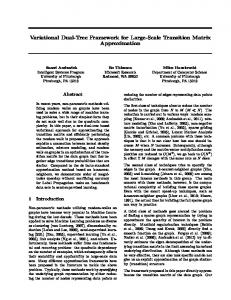
Appendix B. The case of proportionality in the data. We have relegated the discussion on the issue of proportionality among data points to this appendix because it is computationally simple to address but theoretically complex. We will discuss briefly some of the theoretical aspects before we proceed to presenting the modifications of procedure AllPrames needed to adapt it for the case when proportional points are not known to be absent. The assumption of nonproportionality among data points in the data domain appears in previous published works (see e.g., Charnes et al. [1991], expression (8), p. 202 or Dula and Hickman [1997]). This assumption obviates duplication of data points, another common assumption. In a work that deals with all four DEA models - constant, variable, increasing, and decreasing returns - simultaneously, such as the present work, these two assumptions play different roles. The weaker condition of no duplication of data points is necessary for all four cases for the frames to be unique. However, it is sufficient only for the variable, increasing, and decreasing returns models. Uniqueness of the frame is guaranteed for the constant returns model only if there is no proportionality. Refer to Figure 2 to illustrate the impact of proportional points on the four DEA models and on our principal results. This figure depicts the four production possibility sets for the same data domain: A = {a1, a2,a3, a4}. Notice that pairs of points {a2, a3} and {a1, a4} are proportional (the dashed lines serve to emphasize this relation). The frames for V2, V3, and V4 are T2 — {a1, a2, a3, a4}, T3 — {a3,a4}, and F4 = {a1,a2}, respectively, and these are unique. The first important realization is that V1 has two frames: Tl — {a2} and T1 = {a3}. This loss of uniqueness is a consequence of the fact that the points a2 and a3 are a proportional pair; that is, a2 — aa3 where 0 < a ^ 1. This causes the invalidation of Theorems 1 and 3 and the Corollary in Section 2. With proportionality, Theorem 1 is no longer true for the constant returns model and Theorem 3 must be made weaker; i.e.: Fl C (F3 f\ F4). Fortunately for computations, proportional points behave predictably in their relation to frames and can be handled efficiently One reason for this is the fact that if there is a set of two or more proportional points, only the one with the smallest and the one with the largest norm can belong to any of the frames T2,T3,T4 (anything in between is necessarily not extreme-efficient). If a proportional pair belongs to any of these frames at all, then: i) both points in the pair must belong to F2\ ii) the longest of the two necessarily belongs to F3 but not to T4\ and in) the shortest

Duld & Thrall

Page 20

Figure 2. The four production possibility sets from the same data set with proportionality.

a. V: The Variables Returns PPS.

c. V: The Decreasing Returns PPS.

d. V: The Constant Returns PPS.

of the two necessarily belongs to T4 but not to T3. This means that the issue of proportionality becomes relevant only after the three frames, Jr2,^"3, and T4 have been found. Only proportional pairs in T2 which are also efficient with respect to the constant returns model are eligible to. belong in Tl. This is illustrated in Figure 2 with the proportional pair {a2, a3} being an eligible pair while {a1, a4} is not. Exactly one point from each eligible pair ends up in T1. The complication with proportional points is a consequence of the fact that neither from an eligible pair appears in Tz D F4. The example connected with Figure 2 can be used to verify this. Therefore we need to identify eligible proportional pairs in T2 and provide an unambiguous rule for selecting which one from such a pair is to appear in Tx. A rule to distinguish between eligible and ineligible proportional pairs in T2 is a consequence of the following lemma: LEMMA.

Let a*1 and aJ'2 be two points in A such that a-72 = aaP1 for a > 1 and suppose a0 —

7a-71 + (1 — 7)aj2 € S^ for some 0 < 7 < 1. Then aP1,^2, and a0 are all efficient with respect to the constant returns DEA model.


Page 21

Proof. Since a0 is efficient with respect to the variable returns model, there exist 0 < IT* E 3?m, and ß* € 3? such that (ir*,a°)+ß*=0, {Tr*,aj)+ß*