1
Videoshop: A New Framework for Spatio-Temporal Video Editing in Gradient Domain* Hongcheng Wang† , Ning Xu† , Ramesh Raskar‡ and Narendra Ahuja† † Beckman Institute, University of Illinois, Urbana, IL 61801 Email: {wanghc, ningxu, ahuja}@vision.ai.uiuc.edu ‡ Mitsubishi Electrical Research Laboratories (MERL), Cambridge, MA Email:
[email protected]
Abstract— This paper proposes a new framework for video editing in gradient domain. The spatio-temporal gradient fields of target videos are modified and/or mixed to generate a new gradient field which is usually not integrable. We compare two methods to solve this ”mixed gradient problem”, i.e. the variational method and loopy belief propagation. We propose a 3D video integration algorithm, which uses the variational method to find the potential function whose gradient field is closest to the mixed gradient field in the sense of least squares. The video is reconstructed by solving a 3D Poisson equation. The main contributions of our framework lie in three aspects: firstly, we derive a straightforward extension of current 2D gradient technique to 3D space, thus resulting in a novel video editing framework, which is very different from all current video editing software; secondly, we propose using a fast and accurate 3D discrete Poisson solver which uses diagonal multigrids to solve the 3D Poisson equation, which is up to twice as fast as a simple conventional multigrid algorithm; finally, we introduce a set of new applications, such as face replacement and painting, high dynamic range video compression and graphcut based video compositing. A set of gradient operators is also provided to the user for editing purposes. We evaluate our algorithm using a variety of examples for image/video or video/video pairs. The resulting video can be seamlessly reconstructed. Index Terms— video editing, image processing, poisson equation, graphcut, gradient domain.
I. I NTRODUCTION With increasing access to and sophisticated use of digital video camcorders, there is evergrowing interest in video editing tools allowing consumers to manipulate the captured video. While commercially available digital video editing tools such as Adobe Premier [1] and Final Cut [2] by Apple do allow so-called non-linear editing, the pipeline of cutting, pasting, and trimming sequences of frames is reminiscent of traditional physical film cutting. On the other hand, photo editing tools such as Photoshop [3] allow more complex operations on individual images but they cannot be seamlessly applied to videos. Our goal is to develop tools that go beyond frameconstrained manipulation such as resizing, color correction, and simple transitions, and provide object-level operations within frames. Some of our targeted video editing tasks include transferring a motion picture to a new still picture, importing a moving object into a new background, and compositing two video sequences.
The challenges behind this kind of complex video editing tasks lie in two constraints: 1) Spacial consistency: Imported objects should blend with the background seamlessly. Hence pixel replacement, which creates noticeable seams, is problematic. 2) Temporal coherency: Successive frames should display smooth transitions. Hence frame-by-frame editing, which results in visual flicker, is inappropriate. Our work is aimed at providing an easy-to-use video editing tool that maximally satisfies the spatial and temporal constraints mentioned above and requires minimum user interaction. This tool is based on a new approach for video editing in the spatio-temporal gradient domain. A number of different operators are provided for gradient manipulation. As shown in our experimental results, our approach is able to seamlessly perform tasks such as face replacement, moving object insertion, and video compositing. By manipulating the gradient domain representations, a user can edit video sequences in many interesting ways. Figure 1 shows an overview of our approach. All the user needs to do is to give a region of interest (ROI) in step 1 and then select a gradient operator (which will be defined in Section III-A) in step 3. An example of importing a moving person from one lawn to another is shown in Figure 2. After user giving a ROI that contains the moving person and an operator of ’SUBSTITUTE’, the system automatically generates a new video with the moving person in the new background. II. R ELATED W ORK A. Image and Video Editing 1) Image editing: Our work is directly related to existing work on image editing. The Photoshop software has been widely used by consumers. To the best of our knowledge, most of the techniques used in the software have not been published. Since the seminal work by by Porter and Duff [4], there has been an increasing interest in exploring new techniques for image editing due to the wide use of digital cameras. Pyramid based image editing proposed by Adelson et al. [5] decomposes an image into low and high frequency bands, and different frequency bands are combined with different alpha masks for image compositing. Lower frequencies are mixed over a wide region around the boundary, and fine details are mixed in a narrow region around the boundary.
2
2 Input Sequence 1
3
1 Regions of interest
1 Input Sequence 2
3D gradient field
2
Modified 3D field of gradients
4
Output sequence
3D gradient field
Fig. 1. Steps in our approach: 1. Obtain the region of interest (ROI) through user interaction. 2. Calculate the 3D gradient field of the input sequences. 3. Modify the 3D gradient field based on the gradient fields of input sequences. 4. Integrate the modified gradient field to obtain a composite video sequence.
This approach works in pixel domain and the resulting image exhibits a gradual transition along the boundary. Barrett and Cheney [6] propose an object-based image editing method in which the foreground objects are modified interactively at the object level. Tan and Ahuja [7] propose selecting objects with freehand sketches through alpha channel estimation for editing natural images. Recent methods for image editing proposed by P`erez et al. [8] and by Elder and Goldberg [9] work in gradient (contour) space. Images are reconstructed by integrating the modified gradients by solving a Poisson equation. 2) Image/video matting: Our work is also related to research in image/video matting or compositing [10]. The goal of video matting is to insert new elements seamlessly into a scene. Traditional methods like blue-screen matting used for film production require strictly controlled studio environments, and therefore are not suitable for home video editing. A recent method suggested by Chuang et al. [10] overcomes this constraint by segmenting a hand-drawn keyframe into trimaps, and then performing interpolation using forward and backward optical flow. They mainly focus on the exact extraction of an alpha matt from a video sequence, which is difficult but necessary. Finally, some image inpainting algorithms use techniques similar to ours by solving PDEs which are more complex than Poisson equations [11]. 3) Video texture editing: Some work on dynamic texture synthesis and editing is also related to our work. Doretto and Soatto [12] propose modifying the intensity, scale and speed of a single dynamic texture. Graphcut textures [13] combine two dynamic textures by finding the minimum cut between them and then forming a direct composite in image domain. This approach has problems when the two video sequences have differences in camera gain or scene illumination, geometrical misalignments or motion inconsistency. 4) High dynamic range video compression: A conventional digital camera typically provides a dynamic range of two orders of magnitude through the CCD’s analog-to-digital con-
verter (the ratio in intensity between the brightest pixel and the darkest pixel is usually referred to as the dynamic range of a digital image). However, many real-world scenes have a larger brightness variation than can be linearly recorded by the image sensors. Thus, some areas of the images captured by digital cameras are undersaturated or oversaturated. Tonemapping (also called tone reproduction) is an efficient way to faithfully reconstruct high dynamic range radiance on a low dynamic range display. To capture a high dynamic range image, several images with different exposures are usually taken to cover the whole range of a real scene using conventional cameras. Those images are combined into a single high dynamic range image (radiance map). High dynamic range radiance maps are recovered from these images [14] and tonemapping methods are then applied to the radiance maps to reduce the dynamic range. Many tonemapping algorithms for compressing and displaying HDR images have been proposed [15], [16], [17], [18]. Reinhard et al. [18] have achieved local luminance adaptation by using the photographic technique of dodging-and-burning. Tumblin and Turk [17] propose the Low Curvature Image Simplifier (LCIS) by applying anisotropic diffusion to prevent halo artifacts. Fattal et al. [16] propose a method to attenuate high intensity gradients while magnifying low intensity gradients, in which the luminance is recovered from the compressed gradients by solving a Poisson equation. In spite of these efforts on HDR image display, there is limited progress on robust algorithms for tonemapping HDR video. Kang et al. [19] describe an approach which varies the exposure of alternate frames. It requires a burdensome registration of features in successive frames to compensate for motion. Given the feature correspondence problem, rapid movements and significant occlusions cannot be dealt with easily. In addition, the two different exposures may not capture the full radiance map of a scene. More exposures will make the feature registration problem more difficult.
3
Fig. 2. Object Insertion. F IRST ROW FROM LEFT : a selected region of interest, i.e. a mask; original video sequence; new background; S ECOND ROW FROM LEFT : reconstructed video; the person is duplicated in the new background.
B. Gradient-based Techniques Gradient domain techniques have been widely used in computer vision and computer graphics. The motivation to use gradients is based on the retinex theory of Land and McCann [20] which states that the human visual system is not very sensitive to absolute luminances reaching the retina, but rather to illumination differences. A number of applications based on this technique have been developed, such as shadow removal by Finlayson et al. [21]; multispectral image fusion by Socolinsky and Wolff [22]; image and video fusion for context enhancement by Raskar et al. [23]; image inpainting by Ballester et al. [24]; and High Dynamic Range image compression by Fattal et al. [16].
C. Contributions of Our Work In spite of the fast progress in object-level image editing, there has been surprisingly little work done in video editing. One exception is the work presented by Bennett and McMillan [25] where video sequences are treated as a spatiotemporal volume that can be sheered and warped under user control. Their work is still in the original image domain, and as a result importing a new object will result in a ”cutout” effect. Our work extends the gradient based techniques to three dimensional space by considering both spatial and temporal gradients, which leads to more versatile video editing capabilities. Within our framework, we treat a video as a 3D
cube but is in forms of gradient instead of intensity. The main contributions of our work include: 1) Extension of 2D gradient technique to 3D: Though the extension from 2D gradient technique to 3D simply requires the addition of time as another dimension, it leads to a wide range of video editing applications. 2) 3D poisson solver using diagonally oriented grids: We propose using a 3D poisson solver on diagonally oriented grids to solve the 3D poisson equation. The scheme is found to be up to twice as fast as comparable conventional multigrid algorithms. This is important when dealing with videos. This paper is an extended version of our previous conference paper [26]. We present a comprehensive description of our novel video editing framework with systematic analysis of the algorithm and results. In addition, we introduce a set of new applications within this framework, such as face replacement and painting, high dynamic range video compression using split-aperture camera, and video compositing based on automatic mask generation using 3D graph-cuts. III. G RADIENT D OMAIN V IDEO E DITING Current gradient domain methods [16], [8], [21], [22], [23] can be considered as performing 2D integration after modifying the 2D gradient field. The integration involves a scale and shift ambiguity in luminance plus an image dependent exponent when assigning colors. Hence, a straightforward
4
frame by frame application to video will result in a lack of temporal coherency in luminance and flicker in color. We instead treat the video as a 3D cube and solve this problem via 3D integration of a modified 3D gradient field. Consider an extreme example in order to contrast the two approaches. We deliberately set the gradients in a video which are smaller than some threshold to zero. The video obtained via 2D or 3D integration will have a (cartoon like) flattenedtexture effect. The frame by frame 2D integration approach results in noticeable flicker, while the video reconstructed by 3D integration shows near-constant and large flat colored regions. A. Gradient Operators To facilitate editing operations in the spatio-temporal gradient space, we provide a set of gradient operators, O = {MAX , MIN , LINEAR , THRES , ZERO , · · ·, SUBSTITUTE} (1) which are used to compare gradients from different channels, c, or dimensions, ijk (spatial dimension, temporal dimension or both) when editing videos. Assume G1 and G2 are gradients of two source images/videos, G is the target gradient and M is a given mask, we define a set of gradient operators as follows: 1) MAX / MINc,ijk (G1 , G2 , M ) G = max / minc,ijk (G1 , G2 ) · M
(2)
This operator is used to extract large or small spatial/temporal gradients within a mask of two input video sequences. For example, MAXc,k (G1 , G2 , M ) can be used to compare the gradients in the temporal dimension. 2) ZERO(G1 , M ) G = G1 · (1 − M )
(3)
The ZERO operator sets the gradient in the mask region at zero, which can be used for inpainting of small scratches in the film or removing shadows. 3) LINEAR(G1 , G2 , M ) G = (µ · G1 + ν · G2 ) · M
(4)
where µ and ν are weights, and usually µ + ν = 1. The LINEAR operator finds the linear combination of two gradients G1 and G2 . 4) SUBSTITUTE(G1 , G2 , M ) G = G1 · M + G2 · (1 − M )
(5)
The SUBSTITUTE operator simply substitutes G1 with G2 in the mask region. It is often used to insert a foreground moving object into a new background. 5) THRES(G1 , M ) G = (G1 > δ) · M
(6)
where δ is a threshold. The THRES operator is used to extract the gradients which are larger than some usergiven threshold δ. 6) COMPRESS(G1 , M ) G0 = (α/ kG01 k)β · G01 · M
(7)
where, G0 and G01 are defined in the log-domain in spatial domain; α = 0.1 ∼ 0.2 times the average gradient norm of G01 ; β is a constant with a value between 0 and 1. It is similar to the gradient attenuation function as in [16]. The COMPRESS operator is used to attenuate large gradients and magnify low gradients. Thus, it can be used for high dynamic range video compression. Note that if we attenuate the 3D loggradients in a straightforward way, some artifacts may result since the temporal gradients will be attenuated and the motion will be smoothed. This is made obvious by imagining that a ball is moving in a scene. If we compress the temporal gradient of the sequence, the reconstruction of the scene will be blurred. Therefore, we choose to attenuate only spatial gradients. B. 3D Video Integration Our task is to generate a new video, I, whose gradient field is closest to the modified gradient, G. One natural way to achieve this is to solve the equation ∇I = G
(8)
However, since the original gradient field has been modified using one of the operators discussed above, the gradient field is not necessarily integrable. Parts of the modified gradient may violate ∇×G=0 (9) (i.e., violate the requirement that the curl of gradient be 0). Recently, two approaches have been proposed to solve the mixed gradient problem: 1) The variational method: Kimmel et al. [27] propose minimizing a penalty function of image gradient and intensity using a variational framework. A projected normalized steepest descent algorithm was proposed to solve this problem. P`erez et al. [8] and Fattal et al [16] use a similar framework by considering only the image gradient in the penalty function. They solve this problem by finding a potential function I, whose gradients are closest to G in the sense of least squares by searching the space of all 2D potential functions. They use this technique for image editing [8] and high dynamic range image compression [16], respectively. 2) Loopy belief propagation: The essence of this method is to enforce the curl constraint in Equation 9 via loopy belief propagation [28] across a graphical model. A maximum a-posteriori estimate of a potential function can be found via message passing within the graphical model. This method has been used in image phase unwrapping [29] and enforcing the surface integrability for shape from shading [30]. We test these two methods using a simple image editing example. Figure 3 illustrates the comparison. We can see that the variational method results in better results than loopy belief propagation, which has a ”washed-out” effect throughout the whole image. This is mainly because loopy belief propagation propagates the gradients which violate the curl constraint to the
5
Fig. 3. From left to right: input image 1 (mask is not shown); input image 2; compositing result using the variational method; compositing result using loopy belief propagation.
whole image, but the variational method limits the propagation within the mask boundary. Therefore, we choose to extend current variational methods for video editing by considering both spatial and temporal gradients in 3D space. Assuming the mask is represented by Ω, we minimize the following integral in 3D space (hence the reference to 3D video integration in the sequel): ZZ Z f (I) = F (∇I, G)dxdydt (10)
solution of 3D Poisson equation converge fast. In this case, the intensity gradients are approximated by forward difference: I(x + 1, y, t) − I(x, y, t) ∇I = I(x, y + 1, t) − I(x, y, t) /h I(x, y, t + 1) − I(x, y, t) where h is the grid distance. We represent Laplacian as: ∇2 I
= [−6 · I(x, y, t) + I(x − 1, y, t) + I(x + 1, y, t) +I(x, y + 1, t) + I(x, y − 1, t) + I(x, y, t + 1) +I(x, y, t − 1) ] /h2
Ω
where, F (∇I, G)
2
= k∇I − Gk ∂I ∂I ∂I = ( − Gx )2 + ( − Gy )2 + ( − Gt )2 ∂x ∂y ∂t
According to the Variational Principle, a function F that minimizes the integral must satisfy the Euler-Lagrange equation: ∂F d ∂F d ∂F d ∂F − − − =0 ∂I dx ∂Ix dy ∂Iy dt ∂It for all I ∈ Ω. We can then derive a 3D Poisson Equation: ∇2 I = ∇ • G
(11)
where ∇2 is the Laplacian operator, ∇2 I =
∂2I ∂2I ∂2I + 2+ 2 2 ∂x ∂y ∂t
and ∇ • G is the divergence of the vector field G, defined as ∂Gx ∂Gy ∂Gt ∇•G= + + ∂x ∂y ∂t
The divergence of gradient is approximated as: ∇•
G
= [Gx (x, y, t) − Gx (x − 1, y, t) + Gy (x, y, t)− Gy (x, y − 1, t) + Gt (x, y, t) − Gt (x, y, t − 1) ] /h2
This results in a large system of linear equations. We use the fast and accurate 3D multigrid algorithm in [31] to iteratively find the optimal solution to minimize Equation 10. Due to the use of diagonally oriented grids, this algorithm does not need any interpolation when prolongating from a coarse grid onto a finer grid. Actually, a ’red-black’ Jacobi iteration of the residual between the intensity Laplacian and divergence of gradient field avoids interpolation. Most importantly, the speed of convergence is much faster than the usual multigrid scheme. IV. V IDEO E DITING TASKS In this section, we present experimental results using several operators in gradient domain to illustrate various applications of our video editing framework.
C. 3D Discrete Poisson Solver
A. Digital Face Replacement and Painting
In order to solve the 3D Poisson equation (Equation 11), we use the Neumann boundary conditions ∇I · ~n = 0, where ~n is the normal vector on the boundary of mask Ω. For 3D video integration, due to high data volume and increased computational complexity, we need to resort to a fast algorithm. For this purpose, we use a diagonal multigrid algorithm originally proposed by Roberts [31] to solve the 3D Poisson equation. Unlike conventional multigrid algorithms, this algorithm uses diagonally oriented grids to make the
Digital face replacement and painting involves replacing the face of a person in a target image using the face of another person in a source video. The shape, expression and motion of the face in the resulting video will be the same as in the source video, but the color and appearance of the face will be the same as the target face so as to fit in the environment of the target image. Face replacement is different from reanimating faces in image and video as in [32], where the shape and appearance are not changed, but they use 3D models. Our
6
Fig. 4. L EFT: The image of ”the famous fat boy”; R IGHT: Face replacement using photo editing tool. (images from http://www.nei.ch/gallery/famousfatboy)
work is inspired by a recent popular web prank - ”the famous fat boy”, where a boy’s face appears on different pictures by photo editing amateurs. Figure 4 gives an example from this page. An automated system for face replacement and painting has many potential applications, such as Hollywood special effects and personalized movies. Currently, face replacement and painting is usually done manually by graphic artists using photo editing software, such as Photoshop. This is a tedious process even for a single image. It is almost impossible for a video sequence. Using our approach, face replacement becomes as easy as a few mouse clicks. Without using face tracking, we assume the person stays still, and the user is asked to mask the ROI for replacement in the first frame of the source video and input the offsets and scale for the mask to put in the target image. In this case, the ’SUBSTITUTE’ operator is used. Figure 5 shows some examples of face replacement and painting. The face in the source video can be rotated or flipped horizontally in the image plane in order to replace faces in different images. We can perceive the shape of the original face, though its color has been changed. This is because the high gradients in the mouth, eye and nose areas are retained and the low gradient regions surrounding them is more affected by those of new background. As far as we know, we are the first to define the problem of digital face replacement and painting. This is an important issue for artists or cartoonists since they might want to borrow some ideas from different sources when building a new character.
B. Video Compositing Using Gradient Operators In this section, we give several examples of compositing of two videos. To extract motion objects, the layered representation of video sequences [33] can be used according to the affine motion parameters based on the optical flow. We tested our algorithm using the optical flow and temporal gradients for comparison, and there was not much difference visually, though we believe a good optical flow computation could improve our results.
Figure 6 illustrates an example of compositing a fish sequence and a clock sequence. The purpose is to insert the clock into the fish sequence, and at the same time, to make the clock face and the pendulum look transparent. These two regions of interest are selected from user interaction. The MAX operator is used based on the magnitude of both spatial and temporal gradients. The resulting sequence shows the effect of transparency in the regions of clock face and pendulum. Figure 7 shows an example combining two video sequences using the ’THRES’ operator. The purpose is to move the fountain in the fountain sequence to the ocean sequence. We consider the temporal gradient of the fountain sequence. The corresponding gradients in the ocean sequence are replaced by those of the fountain sequence, where the temporal gradients of the fountain sequence are larger than some user given threshold. This is a challenging example due to the non-rigid motion of the fountain. We believe that none of the previous video editing tools can perform this task. The region of interest in this example is the whole image.
C. Graphcut Based Video Compositing To obtain the regions of interest for video compositing, we can also use a 3D graph cut algorithm to find the minimum cut between two sequences, and then use gradients of one video sequence on one side of the cut while using gradients of the other video sequence on the other side. 3D graph cut has been used for spatial or temporal video extensions by Kwatra et al. [13]. As stated in Section II, compositing videos directly from the graph cut results will cause artifacts due to factors such as illumination and appearance. By combining gradient fields on the two sides of the cut, we can apply our 3D integration algorithm to reduce the artifacts significantly. In this paper, we extend the 2D graph cut algorithm presented by Xu et al. [34] to the spatio-temporal space. The implementation is more efficient than usual graph cut algorithm. We provided a variety of operators for this operation, such as horizontal cut, vertical cut, and arbitrary cut. Figure 8 gives an example of image compositing by finding a 2D minimum cut. We use a simple cost function for the
7
Fig. 5. F IRST ROW: (Left) a shifted and scaled mask example; (Right) three frames from original video sequence; S ECOND ROW: replacement of the princess’ face; T HIRD ROW: replacement of the face of the status of liberty (original images are rotated); F OURTH ROW: replacement of the face of President Thomas Jefferson; F IFTH ROW: replacement of the face of Shrek (original images are flipped horizontally).
overlap region (the whole image here), B: c=
X
|G1 (i) − G2 (i)|
2
(12)
i⊂B
where G1 and G2 are spatial gradients of overlap regions of two input images, respectively. Figure 9 gives results obtained using 3D horizontal and vertical minimum graph cuts. We use a cost function consisting
of both spatial and temporal gradients: X 2 2 c= α · |G1 (i) − G2 (i)| + β · |G1t (i) − G2t (i)| (13) i⊂B
where G1t and G2t are temporal gradients of two input sequences, respectively, and α and β are weights of spatial and temporal gradients. For this example we use α = β = 1. We can see that the gradient compositing has much better results than direct intensity compositing along the cut in both examples.
8
Fig. 6. F IRST ROW: fish sequence; S ECOND ROW: clock sequence; T HIRD ROW: reconstructed sequence using maximum temporal gradients has the effect of transparency (multiple masks are used but not shown.)
Algorithm 1: General algorithm for HDR video display Data: LDR video I1 , I2 , . . . , In Result: HDR video I Recover the radiance map; Attenuate large gradients and magnify small ones using COMPRESS operator; Reconstruct new video I by solving a Poisson equation;
D. HDR Video Compression Our video HDR compression problem is stated as follows: Given n synchronized LDR videos, I1 , I2 , . . . , In , with different exposures, find an HDR video, I, which is suitable for typical displays. First, the radiance map from the input videos can be computed using a method such as in [14] for corresponding images in the videos (We will not discuss the details of recovering the radiance map here). Then our task is to generate a new video, I, whose gradient field is closest to the gradient of the HDR radiance map video, G. The general algorithm for HDR video display is described in Algorithm 1. We used the high dynamic video camera called split aperture camera [35] developed to capture the HDR video. The camera uses a corner of a cube as a 3-faced pyramid and three CCD sensors. Three thin-film neutral density filters with transmittances of 1, 0.5 and 0.25 are put in front of the sensors respectively. We used Matrox multichannel board capable of synchronizing and capturing three channels simultaneously.
The three sensors and the pyramid were carefully calibrated to ensure that all the sensors were normal to the optical axes. The setup of our HDR video capture devices is shown in Figure 10. We tested our 3D video integration algorithm for video HDR compression on a variety of scenarios. To maintain Neumann boundary conditions, during preprocessing, we padded the video cube with 5 pixels in each direction. The first and last 5 frames, and first and last 5 row/column pixels of each frame input to the algorithm are all black. The attenuation parameter β in Equation 5 is set to 0.15 in all experiments. Figure 10 shows an example of three videos captured using our camera. Due to the shadow of the trees and strong sunlight, none of the individual sensors can capture the whole range of this dynamic scene. For example, the trees and the back of the walking person are too dark in (a) and (b), but too bright in (c). The light bar in (a) is almost totally dark, and the ground is overexposed in (b) and (c). However, the video obtained using our 3D video integration algorithm can capture almost everything clearly in the scene. The detailed motion of the tree leaves is also visible. As far as the authors know, our approach is the first proposed method for displaying HDR video that does not require inter-frame registration of features with the help of a specially designed camera.
9
Fig. 7. Ocean-Fountain example (color). FIRST ROW: waving ocean sequence 3D video integration algorithm based on the temporal gradient.
Fig. 8.
SECOND ROW :
fountain sequence
THIRD ROW :
reconstructed video using our
From left: input image 1; input image 2; result of gradient compositing using horizontal cut; result of intensity compositing using horizontal cut;
V. D ISCUSSION A. Computational Complexity Analysis The space requirement for 3D discrete Poisson solver is of O(n),where n is number of voxels. 3D Poisson solver with second order accuracy will take O(n) time. (For all examples in Section V, we used 256 × 256 × 256 video sequences, i.e., n = 2563 ). There are around 100 iterations for the convergence with 35.7n flops per iteration. Though this is a little higher than the simple usual multigrid scheme, the proposed scheme is up to twice as fast as comparably simple conventional multigrid algorithms [31]. The computational complexity is of O(n(mn+n log U )) for general graphcut algorithm, where n is the number of nodes, m is the number of edges and U is the largest edge cost.
Since we used a simple topology of the graph as in [34], the algorithm is much faster in practice. Practical study shows that our 3D graphcut algorithm has the complexity of O(n1.2 ).
Our current implementations consists of a 3D graph cut algorithm in C++, and a 3D Poisson solver in Matlab on a Pentium IV 2.4G with 2G RAM. For 256 × 256 × 256 video sequences, 3D graphcut takes about one minute, and 3D video integration takes about 10 minutes. Because many loops are involved in solving the 3D Poisson equation, our C++ implementation speeds up the running time to around 25 seconds.
10
Fig. 9. F IRST ROW: Left: input video sequence 1; Middle: result of gradient compositing using vertical cut; Right: result of gradient compositing using horizontal cut; S ECOND ROW: Left: input video sequence 2; Middle: result of intensity compositing using vertical cut; Right: result of intensity compositing using horizontal cut.
B. Limitations of Our Current Framework Though we have obtained promising results on a set of applications with our proposed novel video editing framework, there are still some limitations: 1) We do not consider the light effects during compositing. For example, in the President example in Figure 5, the shadow is not appropriately generated in face replacement and painting. This is a similar problem as in almost all the image editing tools, and it can not be dealt with without incorporating 3D information of the scene. 2) We assume heads do not move in face replacement and painting. This assumption could be relaxed with rough video registration, or face tracking, or by volume warping and scaling as in [25]. 3) Reconstructing video using 3D gradient integration places high demand on memory and computational time. The proposed framework is still expensive for a reasonably large video. The reconstruction involves volumetric datastructures and solving a large 3D Poisson equation. However, this can be improved by graphics processor (GPU) implementation of multigrid algorithm [36] extended to 3D. VI. C ONCLUSION AND F UTURE W ORK We have presented a new framework for video editing which treats video as a 3D cube of pixels. By manipulating videos in the spatio-temporal gradient domain, our approach provides an object-level editing facility not available in traditional systems. The tool requires minimum user interaction, creates seamless compositing, preserves temporal consistency and avoids artifacts common in frame-by-frame video processing. Finally, we have presented a set of new applications, such
as face replacement and painting, high dynamic range video compression and graphcut based video compositing. Currently we are investigating new methods to preserve temporal consistency, such as two-frame constrained video editing, such that we can process larger resolution videos without loading the whole video into memory. We are also working on extracting reflectance properties and lighting conditions from multiple images, which are in turn used for face relighting [37]. This is important to generate consistent shadows in face replacement. In the future, we plan to investigate more work from theoretical and application points of view in the following aspects: 1) The integrability of mixed gradient fields is still an open problem, and we are interested in studying this problem from theoretical and application aspects. 2) We plan to explore other applications of our gradient domain techniques in video editing, such as video inpainting, video shadow removal, 3D face editing and animation, etc. We believe that our gradient-based approach can provide as versatile editing functions to videos as photoeditors provide for images. (The demo video is available online: http://vision. ai.uiuc.edu/˜wanghc/research/editing.html) R EFERENCES http://www.adobe.com: Adobe Premiere Pro. [1] [2] http://www.apple.com/finalcutpro/: Apple Final Cut Pro 4.0. [3] http://www.adobe.com: Adobe Photoshop 7.0. [4] T. Porter and T. Duff, “Compositing digital images,” computer Graphics, pp. 253–259, July 1984. [5] E. Adelson, C. Anderson, J. Bergen, P. Burt, and J. Ogden, “Pyramid method in image processing,” RCA Engineeer, vol. 29, no. 6, pp. 33–41, November 1984.
11
(a)
(b)
(c) Fig. 10. Experimental results on high dynamic range video. Left row: The three video sequences obtained by split aperture camera; The brightness of the three videos are in ratios 1:2:4; Right row (up): The camera used to capture HDR video; Right row (down): The video obtained using our 3D video integration algorithm. The size of video is 256 × 256 × 35.
[6] W. A. Barrett and A. S. Cheney, “Object-based image editing,” SIGGRAPH’02, pp. 777–784, 2002. [7] K.-H. Tan and N. Ahuja, “Selecting objects with freehand sketches,” In proceedings IEEE International Conference on Computer Vision (ICCV), vol. 1, pp. 337–344, July 2001. [8] P. P`erez, M. Gangnet, and A. Blake, “Poisson image editing,” Siggraph, pp. 313–318, 2003. [9] J. H. Elder and R. M. Goldberg, “Image editing in contour domain,” IEEE Trans. PAMI, vol. 23, no. 3, pp. 291–296, March 2001. [10] Y.-Y. Chuang, A. Agarwala, B. Curless, D. H. Salesin, and R. Szeliski, “Video matting of complex scenes,” SIGGRAPH’02, pp. 243–248, 2002. [11] M. Bertalmio, G. Sapiro, V. Caselles, and C. Ballester, “Image inpainting,” SIGGRAPH’00, pp. 417–424, 2000. [12] G. Doretto and S. Soatto, “Editable dynamic textures,” Proceedings of Conference on CVPR ’03, vol. 2, pp. 137–142, June 2003. [13] V. Kwatra, A. Sch¨odl, I. Essa, G. Turk, and A. Bobick, “Graphcut textures: Image and video synthesis using graph cuts,” ACM Transactions on Graphics, SIGGRAPH, pp. 277–286, 2003. [14] P. Debevec and J. Malik, “Recovering high dynamic range radiance maps from photographs,” SIGGRAPH 97, Aug. 1997. [15] F. Durand and J. Dorsey, “Fast bilateral filtering for the display of highdynamic-range images,” ACM Transactions on Graphics (TOG), vol. 21, no. 3, pp. 257–266, 2002. [16] R. Fattal, D. Lischinski, and M. Werman, “Gradient domain high dynamic range compression,” ACM Transactions on Graphics (TOG), vol. 21, no. 3, pp. 249–256, July 2002. [17] J. Tumblin and G. Turk, “LCIS: A boundary hierarchy for detailpreserving contrast reduction,” Proc. ACM SIGGRAPH, pp. 83–99, 1999. [18] E. Reinhard, M. Stark, P. Shirley, and J. Ferwerda, “Photographic tone reproduction for digital images,” SIGGRAPH, pp. 267–276, 2002.
[19] S. Kang, M. Uyttendaele, S. Winder, and R. Szeliski, “High dynamic range video,” SIGGRAPH’03, vol. 61, pp. 1–11, 2003. [20] E. Land and J. McCann, “Lightness and the retinex theory,” J. Opt. Soc. Am., vol. 61, pp. 1–11, 1971. [21] G. Finlayson, S. Hordley, , and M. Drew, “Removing shadows from images,” ECCV, pp. 823–836, 2002. [22] D. Socolinsky and L. Wolff, “A new visualization paradigm for multispectral imagery and data fusion,” CVPR, vol. 1, June 1999. [23] R. Raskar, A. Ilie, and J. Yu, “Image fusion for context enhancement,” NPAR’04, 2004. [24] C. Ballester, M. Bertalmio, V. Caselles, G. Sapiro, and J. Verdera, “Filling-in by joint interpolation of vector fields and gray levels,” MM’03, pp. 2–8, November 2003. [25] E. P. Bennett and L. McMillan, “Proscenium: A framework for spatiotemporal video editing,” MM’03, pp. 2–8, November 2003. [26] H. Wang, R. Raskar, and N. Ahuja, “Seamless video editing,” International Conference on Pattern Recognition (ICPR), 2004. [27] R. Kimmel, M. Elad, D. Shaked, R. Keshet, and I. Sobel, “A variational framework for retinex,” HPL-1999-151R1, 1999. [28] J. Yedidia, W. Freeman, and Y. Weiss, “Generalized belief propagation,” Advances in Neural Information Processing Systems, 2001. [29] B. J. Frey, R. Koetter, and N. Petrovic, “Very loopy belief propagation for unwrapping phase images,” Neural Information Processing Systems Conference (NIPS), 2001. [30] N. Petrovic, I. Cohen, B. Frey, R. Koetter, and T. Huang, “Enforcing integrability for surface reconstruction algorithms using belief propagation in graphical models,” IEEE Conference on Computer Vision and Pattern Recognition (CVPR), 2003. [31] A. Roberts, “Fast and accurate multigrid solution of poissons equation using diagonally oriented grids,” Numerical Analysis, July 1999.
12
[32] V. Blanz, C. Basso, T. Poggio, and T. Vetter, “Reanimating faces in images and video,” EUROGRAPHICS’2003, vol. 22, no. 3, 2003. [33] J. Y. Wang and E. H. Adelson, “Layered representation for motion analysis,” CVPR, pp. 361–366, 1993. [34] N. Xu, T. Yu, and N. Ahuja, “Interactive object selection using s-t minimum cut,” Proceedings of Asian Conference on Computer Vision, vol. 3, January 2004. [35] M. Aggarwal and N. Ahuja, “Split aperture imaging for high dynamic range,” Proc. International Conference on Computer Vision (ICCV), pp. 10–17, July 2001. [36] J. Bolz, I. Farmer, E. Grinspun, and P. Schr¨oder, “Sparse matrix solvers on the GPU: Conjugate gradients and multigrid,” SIGGRAPH, pp. 917– 924, 2003. [37] T. Yu, H. Wang, N. Ahuja, and W.-C. Chen, “Sparse lumigraph relighting by illumination and reflectance estimation from multi-view images,” Eurograpics Symposium on Rendering (EGSR), 2006.