Journal of Optimization in Industrial Engineering 17 (2015) 1-10
A New Fuzzy Stabilizer Based on Online Learning Algorithm for Damping of Low-Frequency Oscillations Ali Ghasemia,*, Mohammad Javad Golkarb, Mohammad Eslamic a
Instructor , Young Researchers and Elite Club, Ardabil Branch, Islamic Azad University, Ardabil, Iran b MSc, Department of Control, Imam Mohammad Bagher University, Sari, Iran C MSc, Department of Electrical and Computer, College of Engineering, Khash branch, Islamic Azad University, Khash, Iran Received 11 March, 2014; Revised 20 August, 2014; Accepted 14 October, 2014
Abstract A multi objective Honey Bee Mating Optimization (HBMO) designed by online learning mechanism is proposed in this paper to optimize the double Fuzzy-Lead-Lag (FLL) stabilizer parameters in order to improve low-frequency oscillations in a multi machine power system. The proposed double FLL stabilizer consists of a low pass filter and two fuzzy logic controllers whose parameters can be set by the proposed multi objective optimization process. A multilayer adaptive network is employed to design the fuzzy logic controller with selflearning capability that does not require another controller to tune the fuzzy inference rules and membership functions. In the proposed online learning algorithm, two artificial neural networks are employed which this system makes the FLL stabilizer adaptive to changes in the operating conditions. Therefore, variation in the power system response, under a wide range of operating conditions, is less compared to the system response with a fixed-parameter conventional controller. The effectiveness of the proposed stabilizer has been employed by simulation studies. The effectiveness of the proposed stabilizer is demonstrated on Two-Area Four-Machine (TAFM) power system under different loading conditions. Keywords: Online learning algorithm, Multi objective optimization, Multi machine, Small signal stability, HBMO, Fuzzy stabilizer.
1. Introduction have been developed and many optimization techniques such as Gradual Self-Tuning Hybrid Differential Evolution (GSTHDE) (Wang, 2013), Fuzzy Gravitational Search Algorithm, improved Time Variant Particle Swarm Optimization (TV-PSO) (Shayeghi et al., 2011), Improved Honey Bee Mating Optimization (Shayeghi et al., 2011), PSO-IIW (Ghasemi et al., 2012) etc. have been used to find the optimum set of parameters to effectively tune the PSS. However, Classical PSS (CPSS) cannot have optimal performance for many different operating conditions (Mishra et al., 2012). Thus, a lot of intelligent algorithms have been introduced for optimal parametertuning of the CPSSs (Shayeghi et al., 2014; Mostafa et al. 2012; Abd-Elazim et al., 2013). To expand a high-performance PSS for a wide range of working conditions, fuzzy logic controller (FLC) and Neural Nets (NNs) techniques have been introduced in (Baek et al., 2008; Park et al., 2005). A controller using a high level of concept without requiring a mathematical model of the system to be controlled can be designed using FLC. This controller applies a feasible option to arrest the qualitative and approximate aspects of human
Power System Stabilizer (PSS) as accompanying controllers are used to damp the electromechanical oscillations of the generators in the power systems. The Conventional PSS (CPSS) based on a transfer function and a linear form of the plant for a particular operating point has been widely used (Gonzalez et al., 2008). On the other hand, naturally power systems are known as a dynamic and highly nonlinear structure. Therefore, CPSS performance may deteriorate under variations that result from nonlinear and time-variant characteristics of the controlled plant (Ghasemi et al., 2013). In other words, to reduce the small signal instabilities caused by the Automatic Voltage Regulator (AVR) and other factors, the PSS was introduced to stabilize the system and increase the system’s security. On the other hand, the use of PSS is the most widespread strategy used today. Power system stability may be broadly defined as that property of a power system that enables it to remain in a state of operating equilibrium under normal operating conditions and to regain an acceptable state of equilibrium after being subjected to a disturbance (Shayeghi et al., 2012). In the recent research, several techniques of tuning PSS * Corresponding author Email address:
[email protected]
1
Ali Ghasemi et al./ A New Fuzzy Stabilizer Based on Online Learning...
reasoning and decision-making process to control a power system. Also, Artificial NNs (ANNs) have the ability of learning and adaptation. This attribute is required when the complexity of a problem or the uncertainty thereof prevents a priori specification of a satisfactory solution. Furthermore, to tackle the drawback of CPSSs in capturing the nonlinearities in power systems, Fuzzy Logic Controller (FLC) is proposed in the literature (Noshyar et al., 2013; Shayanfar et al., 2011). Shabib (2012) explains the design and tracking performance of a fuzzy PID stabilizer. It is expanded by first relating discrete-time based on PID scheme, and then increasingly deriving the stages needed to integrate a FLC scheme into the PID-type stabilizer. In (Dounis et al., 2013) a new fuzzy-PID stabilizer is presented via incorporating an optimal fuzzy reasoning into a PID stabilizer. Nevertheless, dealing with a complex nonlinear system, the adaptation and self-tuning of PID stabilizers is still a difficult task. Moreover, when a large fault happens, the power system operating points may vary considerably in a nonlinear way, affecting the power system performance. To overcome these issues, a new stabilizer needs to be designed which is capable of capturing the nonlinearities occurring in the power system. To use the advantages of FLC into CPSS stabilizer, this paper presents a Fuzzy-Lead-Lag (FLL) stabilizer to damp low-frequency oscillations in a multi-machine power system. In the introduced control pattern, an FLC is designed to adaptively adjust the parameters of FuzzyLead-Lag (FLL) controllers at each control time step. The advantage of the FLL stabilizer is confirmed via comparison with other controllers in recent scientific researches. Also, the perviously-reviewed heuristic algorithms have many disadvantages associated with them such as insecure convergence, the piecewise quadratic cost approximation and may even fail to converge due to inappropriate initial conditions when the system has a highly epistatic objective function (i.e. where parameters being optimized are highly correlated), and the number of variables to be optimized is large. HBMO is a relatively new heuristic algorithm that has been empirically shown to perform well on many of these optimization problems (Ghasemi, 2013; Javidan et al., 2012). Unfortunately, the standard HBMO algorithm often converges to local optima, especially while the problem has high local optima and constraints. In fact, standard HBMO greatly depends on its parameters adjustments, and it often converges to the local optima so as to be premature convergence. Therefore, some modification has been required for the standard HBMO algorithm to improve its performance. Thus, in this paper, some investigations are presented which indicate that the performance of the HBMO algorithm would be improved efficiently. Therefore, the flow of the proposed controller to damp
electromechanical oscillations can be defined with this structure. The control structure consists of an adaptive FLL stabilizer to track the dynamic characteristics of the plant, and a multi objective online learning HBMO algorithm employed for tuning of controller’s parameters to damp the oscillations of the power system. The rest of the paper is organized as follows; Section 2 provides mathematical formulation of the non-linear multi machine and FLL structure. Section 3 introduces the original HBMO and proposed algorithms. To demonstrate the advantages of the proposed algorithm in the design robust FLL problem, the proposed algorithm is applied to 4-machine 2-Area standard power system; results and comparison with reported results are brought in section 4. Finally, the paper is concluded in Section 5.
2. Dynamic Modeling 2.1. Generator Modeling The nonlinear dynamics of the synchronous generator can be expressed as a set of five first-order linear differential equations given by Eqs. (1)–(5) (Ghasemi et al., 2013). b ( 1) (1) (Pm Pe D ( 1)) M (2) Eq (E fd ( x d x d )i d E q ) T do
(3)
E fd ( K A (v ref v u ) E fd ) T A
(4) (5)
T e E q i q ( x q x d ) i d i q
where, id and iq are d-q components of armature current, Efd, E'd and E'q the voltage proportional to field voltage, the damper winding flux and field flux, respectively. T'd0, T'q0, and u are d-axis and q-axis transient time constants, and the regulator of the excitation system, respectively. In this study, the 4generator 11-bus New England/New York interconnected system with, as shown in Fig 1, is used for simulation. Area 1 1
Area 2
6
5 25Km
G1
7 10Km
C1 L1
110Km
8 110Km
9
3
2.5 11 10Km 25Km
G3
C2 L2
2
4 G2
G4
Fig. 1. One-line diagram of the test system
In this test system, each area contains of two generators with 900 MVA and 20 kV. Each of the units is connected through transformers to the 230 kV transmission line. There is a power transfer of 400MW
2
Journal of Optimization in Industrial Engineering 17 (2015) 1-10
from area 1 to area 2. The detailed bus data, line data, and the dynamic characteristics for all machines, exciters and loads are pointed out in (Shayeghi et al., 2012).
washout block, for the range of oscillation frequencies normally encountered, is negligible.
2.2. Power System Stabilizer (CPSS) The PSS usually uses shaft speed, active power output or bus frequency as input. The PSS mainly consists of two lead-lag filters as shown in Fig. 2. Δω
3. The Proposed Algorithm 3.1. Standard HBMO In this section, the standard (single-objective) HBMO is briefly reviewed. Interested readers are referred to (Shayeghi et al., 2012 for more details. The mating flight between queen and best drone can be described using an annealing function as:
VSMax
STw 1 STw
K PSS
(1 ST1 )(1 ST 3 ) (1 ST 2 )(1 ST 4 )
Upss VSMin
prob (Q , D ) e (f ) S (t ) (7) where Prob (Q, D) is the probability of adding the sperm of drone D to the spermatheca of queen Q (successful mating), ∆(f) the absolute difference between the fitness of D (i.e. f (D)) and the fitness of Q (i.e. f (Q)) and S(t) the speed of the queen at time t. After each mating in space, the queen’s speed S(t) and energy E(t) decay using the following equations: (8) S t 1 S t , 0,1
washout Fig. 2. Structure of PSS
The PSS parameters to be optimized in this paper are the time constants T1,..., T4 and gain KPSS. In this paper, Tw = 10 s is chosen for all controllers. This choice ensures that the phase-lead and gain contributed by the washout block, for the range of oscillation frequencies normally encountered, is negligible (Ghasemi et al., 2013). 2.3. Fuzzy-Lead-Lag (FLL) Stabilizer The main aim for wide area control in power system is selection of control inputs. According to the best of the authors’ knowledge of the pervious works, they used linearized time-invariant system form around a given operating condition to select stabilizing signals for PSSs, but we considered nonlinear system model with sample input signal, speed divisions (Lu et al, 2013). This paper applies FLL stabilizer to offer suitable control signals to the PSS, as shown in Fig. 3.
(1 ST3 ) u FLC 2 (1 ST4 )
du/dt Δw
Out1
(1 ST1) u FLC 1 (1 ST2 ) Out 2
K FLL
u gain
E t 1 E t γ
u max STw uoutput 1 STw
u min
Fig. 3. FLL control configuration.
This FLL stabilizer is described by the following transfer functions: STw (1 ST1 ) uoutput [ .Out 2 1 STw (1 ST 2 ) (6) (1 ST 3 ) .Out1 K FLL .w ] (1 ST 4 ) where, uoutput is the output signal control. KFLL denote the gain of input signal. Typical ranges of the optimized parameters are [0.01-20] for KFLL and [0.01-3] for T1,…, T4. Also, Tw = 5 s is chosen for all controllers. This choice ensures that the phase-lead and gain contributed by the
, 0,1
(9)
The main steps of the HBMO algorithm are given below: Step 1: Initial: this step consists of some sub-routines namely; set parameters for HBMO algorithm, generate random population according to optimization problem and select best answer to the queen. The algorithm starts with the mating–flight, where a queen (best solution) selects drones stochastically to form the spermatheca (list of drones). A drone is then randomly selected from this list for the creation of broods. Step 2: Mating flight: The algorithm starts with the mating flight by Eq. (7). The necessary conditions for the end of mating are when the spermatheca (the queen’s spermatheca size representing the maximum number of mating per queen) is full, or when the energy and speed of the queen (or their thresholds) is (nearly) zero. Step 3: Generation of Children (global search): In this step children are born based on the Eq (10). This step transfers the genes of drones and the queen to the jth individual based on: (10) Brood Drone (Queen Drone ) where, β is the decreasing factor ( 0,1 ). Step 4: Adaptation of Broods: The population of broods is improved by applying the mutation operators as follows: Brood ik Brood ik ( )Brood ik , [0,1], 0 1 (11) Step 5: Checking the termination criteria: If the termination criteria are satisfied, then stop the algorithm, otherwise when new queen from next iteration is better than the previous queen, replace them and go to stage 2.
3
Ali Ghasemi et al./ A New Fuzzy Stabilizer Based on Online Learning...
Otherwise select the current queen and go to stage 2.
number between 0 and 1. Step 3: Mapping the decision variables Step 4: Convert the chaotic variables to the decision variables Step 5: Evaluate the new solution with decision variables.
3.2. Improved HBMO base Local search and mating factor In the standard HBMO, a suitable set of the queen's speed reduction coefficient provides a balance between global and local exploration and exploitation, and the results in less iteration on average to find a properly optimal solution. Hence, a new parameter adjustment system for the HBMO concept called improved HBMO with time varying vital parameter i.e.: queen's speed reduction coefficient is developed in this paper. The motivation for using this technique is improving the global search in the early stage of the optimization stages and cheering the particles to converge toward the global optima at the end of it. In the IHBMO algorithm the speed reduction factor (α) is updated for calculation of queen’s speed in Eq. (7) at each generation as follows: (t ) (Cap cap (t )) / Cap (12) where, Cap is the spermatheca size; cap(t) is the total number of drones selected for mating during the first t transitions. Also, HMO method has gained much attention and widespread applications in different optimization fields. However, it often converges to local optima. In order to overcome this shortcoming, we combined HBMO with chaotic local search (CLS). Therefore, we propose a novel chaos theory, which is given by: c ij1
k 1 k 1 gbest gbest j j 2c i (1 + g k ) cos(2 g k ), 0.5 c i 1 best best k 1 0.1c j (1 cos((1 + gbest ))), 0 c j 0.5 i i k gbest
3.3. Learning Method The main part for all algorithms is diversity so that drawback of some of them is due to the lack of diversity which may not be able to efficiently exploit and explore the search space. In other words, standard HBMO greatly depends on its parameters adjustments, and it often suffers from the difficulty of being trapped in the local optima so as to be premature convergence. To develop the overall effectiveness and performance of the HBMO algorithm, a learning mechanism for brood mutation (escape from local optima) is proposed to tune the grow factors. The control procedure can be employed in local or global diversity performance. Thus, we can consider four aspects in controlled diversity, namely, (i) global, (ii) local, (iii) global random and (iv) local random. The proposed algorithm for optimization problem can be summarized as: Step 1: Calculate the objective functions based on the current drones. Step 2: The proposed networks are trained following the generation point by using the drones in the previous and current drones and their cost objective functions values. Firstly, εHBMO and δHBMO estimated with first training network and the second network is trained for βHBMO estimation. For this learning mechanism, drones in the colony are used as the input data and the output data is their cost function values. The proposed mutation based on Eq (17) is employed to the best drone and sequential neural network colony including Ts drones is created. 1 if t n fr 1 D i , j (t ) D ej (t )[1 ( rand ) ] 2 0 if t n fr (17)
(13)
where, gkbest is the best optimal value for kit iteration k 1 k and g best g best represents the fine tuning necessary to achieve the desired sequence of gyrations. The chaotic local search on the HBMO algorithm can be summarized as follows: Step 1: Generate an initial chaos population randomly for CLS. X cls0 [X cls1 ,0 , X cls2 ,0 ,..., X clsNg,0 ]1N g cx 0 [cx 01 , cx 02 ,..., cx 0Ng ] cx 0j
X clsj ,0 Pj ,min Pj ,max Pj ,min
i 1, 2,..., q
, j 1, 2,..., Ng
where, the chaos variable can be generating as follows: X [X cls1 ,i , X cls2 ,i ,..., X clsNg,i ]1N g , i 1, 2,..., N chaos (15) x clsj ,i cx ij1 (Pj ,max Pj ,min ) Pj ,min , j 1, 2,..., N g Step 2: Determine the chaotic variables cx i [cx i1 , cx i2 ,..., cx iNg ], i 0,1, 2,..., N choas j 1, 2,..., Ng
n 1, 2,...
where, µ denotes a user-defined amplitude coefficient, fr shows the performance frequency, the base vector De is the global best called best drone of the colony, and q is the maximum number of new drones locally produced. Their objective functions values (ObjNN) are estimated by using neural nets (NNObj(Ts)). The drones are sorted based on Non-Dominated Sort (NDS) (Shayeghi et al., 2012 in rising order depending on the objective functions values. The best d drones of Threshold (Ts) are randomly located into the new drone to be used as candidates at the next step of the method as follows:
(14)
i cls
cx ij1 base CLS
j 1, 2,..., d
(16)
j 0
cx rand (0) where, Nchaos is the number of individuals for CLS. Cxi Ng is the ith chaotic variable. Rand() generate a random
4
Journal of Optimization in Industrial Engineering 17 (2015) 1-10
NP 4 t sim
Obj NN NN Obj (T s ) [Obj NN order ] NDS (Obj NN )
4
2 2 2 OS1 j 2 OS 34 2 ) t (1 j 34 )dt max( i 1 j 2 j 2
J1 0.01
0
(18)
(22)
D k (t ) T s (order (i )), k rand [1 s ]
Np Ng
i 1, 2,..., d
J2
max[Re( j 1 i 1
3.4. Fuzzy decision For practical applications, it is important to select one solution, which will satisfy the different goals to some extent. Fuzzy set theory has been implemented to derive efficiently a candidate Pareto optimal solution for the decision makers [19]. Upon having the Pareto optimal set, the proposed approach presents a fuzzy-based mechanism to extract a Pareto optimal solution as the best compromise solution. Usually, a membership function for each of the objective functions is defined by the experiences and intuitive knowledge of the decision maker. In this work, a simple linear membership function was considered for each of the objective functions. The membership function is defined as: f i max f i i max (19) f i f i min
i,j
i ,j
) min{ | Im(i , j ) | }]
(23) where, NP, Ng, tsim, λ and ζ are number of operating condition, number of generators, the time of simulation¸ the ith eigenvalue of the system at an operating point and the desired minimum damping, respectively. α and β are 0.56 and 0.085, respectively. The optimal proposed controller tuning parameters problem can be formulated as the following constrained optimization problem, where the constraints of the FLL stabilizer can be expressed as: Minimize [J1,J 2 ] Subject to : (24) K min K K max T i min T i T i max Also, in the proposed optimization process based on Eqs (22) and (23), each agent is shaped to exhibit the Membership Functions (MFs) of the fuzzy logic controller’s inputs and outputs. For this tuning of MFs, multi scheme with n input is considered which is denoted by m1, m2,.., mn. For this tuning some assumptions are considered that can be scheduled as follow: i) All MFs are defined as guassin partitions with seven segments from -1 to 1. Zero is the center membership function which is centered at zero. ii) Scaling factors of input/output are optimized using the proposed algorithm. The above assumptions are shown in Fig. 4. P1 P2 P3 0 (a)
i 0 0 (20) FDM i i 0 i 1 1 i 1 min where, fi and fimax are the maximum and minimum values of the ith objective function, respectively. For each non-dominated solution k, the normalized membership function FDMk is calculated as: Nobj k FDM i FDM k M i 1Nobj (21) j FDM i j 1 i 1 where M is the number of non-dominated solutions, and Nobj is the number of objective functions.
NB
4. Optimal Tuning of Proposed Control Strategy
NM NS
W1
W2
ZO PS
W3 W4
NB: Negative Big NS : Negative Small PM: Positive Medium
The proposed fuzzy stabilizer design is formulated as a multi objective problem to optimize a conflict set of objective functions comprising the damping factor, and the damping ratio of the lightly damped electromechanical modes, and the effectiveness of the suggested technique is confirmed through eigenvalue analysis and nonlinear simulation results. Two additional objective functions that allowed some eigenvalues to be shifted to the left-hand side of the vertical line in the complex plane or to a wedge-shape sector in the complex plane were further investigated in (Ghasemi et al., 2012). The objective functions for optimization defined by,
PM PB
NM: Negative Medium PS : positive Small PB : Positive Big
(b) S 1 [ P11 P19 W 11 W 112 S2
SF11 SF12
[ P21 P29W 21 W 212
SF21 SF22
[ Pn 1 Pn 9 W n 1 W n 12
SFn 1
SF13 SF23
*] *]
Sn
SFn 2 SFn 3
n : Population size SFij: Scaling factor Pij : Center of the MFs * : Operator code Wij : Width of the MFs Fig. 4. (a) Symmetrical membership functions, and (b) String architecture for tuning membership functions and scaling factors
5
*]
Ali Ghasemi et al./ A New Fuzzy Stabilizer Based on Online Learning...
The combination between optimization FLC is as follow: i) The variables are the standard deviation and mean value of each fuzzy MFs. ii) These variables act as solutions and search for the global best fitness. iii) It starts with an initial set of variables. iv) After the variables had been tuned by the proposed algorithm, these variables will be used to check the
performance of the FLC. v) This process is repeated until the goal is achieved. Figure 5 shows the flowchart of the multi objective online learning HBMO algorithm for optimization. Also, in order to acquire better performance, number of queens, drones, broods, workers, the queen’s spermatheca size are chosen as number of dimension, 40, 25, 15 and 35, respectively.
START Set Algorithm Parameters and Data of test system Generate the initial population based on state variable and chaos initialization
Is termination Criteria satisfied?
Determine new positions for colony
Yes No
Calculate nectar amounts Based on the objective function values
J1
End
J2
Select best answer by fuzzy decision and done NDS sorting for all data Memorize the position of best Queen All Drones Distributed? No
Yes Substitute the new best solution with the previous solution
The procedures of CLS
Keep the previous best solution
Determine new positions based on generation Equation
Is the new best solution better than the previous one?
No
Yes
Fig. 5. Flowchart of the proposed algorithm Table 1 Operating conditions (TAFM) G1 Conditions NO P Q 1 0.7778 0.1021 2 1.084 0.3310 3 0.7778 0.0502 4 0.7778 0.1021 5 6 7
G2 G3 P Q P Q 0.7777 0.1308 0.7879 0.0913 0.7778 0.4492 0.7879 0.1561 0.2333 0.0371 0.7989 0.0794 0.7777 0.1308 0.7989 0.0903 Other Characteristics 20% increase load 20% decrease load 2 line tripe: 7-8, 8,9
The performance of power systems equipped with FLL stabilizer is validated for four-machine two-area study system as given in Fig. 1. Different operating conditions are analyzed for the TAFM power system, as given in Table 1. Figure 6 shows MFs shape of FLL controller
G4 P 0.7778 0.7778 0.7778 0.7778
Q 0.0918 0.2501 0.0704 0.0981
tuned by the proposed algorithm. Figure 7 shows the minimum fitness functions evaluating process. The optimum FLL parameters are given in Table 2 for TAFM power system. Table 2 shows optimum value for FLL controller.
6
NS
Z0
PS
PM
PB
0.8 0.6 0.4 0.2 0 -1
-0.5
0 input1
0.5
1
NB 1
NM
NS Z0
PS
PM
PB Degree of membership
NB NM 1
Degree of membership
Degree of membership
Journal of Optimization in Industrial Engineering 17 (2015) 1-10
0.8 0.6 0.4 0.2 0 -1
-0.5
0 input1
0.5
1
NB 1
NM
NS
Z0
PS
PM
PB
0.8 0.6 0.4 0.2 0 -1
-0.5
0 input1
0.5
1
Fig. 6. Optimized output MFs for proposed algorithm based FLL controller
system were performed using Matlab® and Simulink® software. To assess the robustness and effectiveness of the proposed controller, simulation studies are carried out for various fault disturbances and fault clearing sequences for two scenarios through the nonlinear time simulation and some performance indices using the following stabilizer designing techniques: 1. Classical PSS stabilizer (Shayeghi et al., 2012). 2. PSS stabilizer tuned by Strength Pareto algorithm tuned (Yassami et al., 2010). 3. Proposed Strategy.
3.02
J2
2.79
2.35
1.98 1.65 1.86
1.91
1.98
J1
2.97
2.13
5.1. Scenario I In this scenario, the performance of the proposed stabilizer under transient conditions is verified by applying a 6-cycle three-phase fault at bus 7 at the end of line 7#8. The fault is cleared by permanent tripping of the faulted line. Figure 8 shows oscillations response for G1, G2, G3 and G4 in the introduced fault, under normal operating condition. Assessment of these figures reveals that by using the proposed algorithm the speed deviations of all machines are greatly reduced, have small overshoot, undershoot and settling time.
Fig. 7. Pareto-optimal fronts with proposed algorithm Table 2 Optimal parameters for TAFM test system Parameters Gen KFLL T1 T2 T3 T4 G2 19.63 12.72 0.122 0.291 0.627 G3 19.62 8.534 0.287 0.732 0.194
To demonstrate performance robustness of the proposed algorithm, two performance indices: the ITAE and FD based on the system performance characteristics are defined as:
5.2. Scenario II In this scenario, the performance of the proposed controller tuning under transient conditions is verified by applying a 6-cycle three-phase fault at bus 7 at the end of line 7#8 without line tripping and the original system is restored upon the clearance of the fault. Also, A 20% pulse disturbance in the reference voltage of G1 for 100 ms has been applied. Also, as a large signal disturbance, both the 20% pulse disturbance in the reference voltage of G1 for 100 ms and single phase earth fault on Area 2 bus bar has been applied for 6 cycles. The system response is shown in Fig. 9 for different cases. It can be seen that the proposed technique has good performance in damping of the low frequency oscillations and stabilizes the system quickly.
N G t sim
ITAE
t .(|
i
|).dt
(25)
i 1 0
NG
((600 OS FD
2
i
2
2
) (8000 US i ) 0.01 T s ,i )
i 1
NG
(26)
where, overshoot (OS), undershoot (US) and settling time (Ts) of rotor angle deviation of machine is considered for evaluation of the FD index. Note that the lower value of these indexes shows that the system responds better in terms of time domain characteristics. 5. Simulation and Discussion For arrangement of the introduced design scheme, nonlinear time domain structures of the considered power
7
Ali Ghasemi et al./ A New Fuzzy Stabilizer Based on Online Learning...
x 10
-4
6
Proposed Controller base on ref [14] CPSS Without Controller
5
0
-5 0
4 6 Time (Sec)
-3
8
0 -2 0
10
10
4 2 0 -2 0
2
4 6 Time (Sec)
8
-3
2
w3-w4 (rad/sec)
w1-w4 (rad/sec)
6
2
x 10
x 10
4
w1-w3 (rad/sec)
w1-w2 (rad/sec)
10
2 x 10
8
10
5
0
-5 0
10
4 6 Time (Sec)
-4
2
4 6 Time (Sec)
8
10
8
10
Fig. 8. TAFM system response under nominal condition in scenario I -3
-3
x 10
6 Proposed Controller base ref [14] CPSS Without controller
0.5 0 -0.5 -1 0
2 -3
6
x 10
4 6 Time (Sec)
8
w1-w3 (rad/sec)
w1-w2 (rad/sec)
1
x 10
4 2 0 -2 0
10
2
4 6 Time (Sec)
-3
2
x 10
w3-w4 (rad/sec)
w1-w4 (rad/sec)
1.5 4 2 0
1 0.5 0 -0.5 -1
-2 0
2
4 6 Time (Sec)
8
10
-1.5 0
2
4 6 Time (Sec)
8
10
Fig. 9. TAFM system response for scenario II 20
5.3. Eigenvalues analyze To reveal the performance of the proposed design control for small signal stability, consider Scenario II as a large signal disturbance. The dominant eigenvalues are shown in Fig. 10. A slant black line area and a slant blue line area in this figure shows that the eigenvalues in these areas have a peculiar oscillation between 2.5 and 4.4 (rad/s) (inter-area mode oscillations) and 4.4 and 12.5 (rad/s) (local mode oscillations) respectively. The result of the eigenvalues analysis represented that the proposed method has two inter-area modes and four local modes. When these modes are stabilized, the power system stability is improved. In other words, the results of the proposed controller shows that, the minimum damping ratio and the maximum damping factor, under all cases are better than other methods. Also, the mentioned figure not only depicts that the proposed strategy can shift the unstable or lightly damped oscillation modes but also can shift other oscillation modes more to the left in the splane.
Local mode oscillations
15 10
Inter-area mode oscillations
5
Proposed Controller Ref [14] CPSS without controller
0 -5 -10 -15 -20 -20
-18
-16
-14
-12
-10
-8
-6
-4
-2
0
2
Fig. 10. System dominant eigenvalues for Scenario II in TAFM test system
Also, to have a better comparison between these stabilizers, defined some different operating conditions as shown in Table 3. The electromechanical modes without PSSs for the four cases are tabulated in Table III. It can be seen that these modes are poorly damped, and some of them are unstable (can find with bold format in Table III). The electromechanical modes with the proposed stabilizer are given in Table III, too. It can be found that the electromechanical modes of the base case with the
8
Journal of Optimization in Industrial Engineering 17 (2015) 1-10
proposed PSSs have been shifted to the left-hand side of s-plane. It is obvious that the system damping greatly improved.
work. 100
40
1: Base Case 2: 20% increase 3: 20% decrease 4: 2 line tripe
90
Method
Table 3 Eigenvalues Without and with The Proposed FLL stabilizer
35
Proposed Controller CPSS without controller
80 30 70
Proposed Controller
CPSS
25
Without Controller
60 20
Base Case
-20% Load
2.901i 1.840i 1.140i 1.881i 1.063i 1.103i 1.029i 3.066i 2.874i 2.867i
1.758 ± 4.995i -2.241 ± 2.552i -2.547 ± 2.269i -1.054 ± 1.911i -0.813 ± 1.253i 0.055 ± 1.119i -0.184 ± 1.172i -2.126 ± 3.154i -2.948 ± 0.973i 0.011 ± 0.163i
-1.877 ± -1.456 ± 2.878 ± 2.832 ± -0.397 ± -0.815 ± -0.772 ± -2.173 ± -2.871 ± 0.010 ±
0.013 ± 0.156i
-0.003 ± 0.050i
-0.007 ± 0.010i
-2.467 ± -2.733 ± -1.334 ± -1.793 ± -0.537 ± -0.939 ± -0.478 ± -2.424 ± -2.416 ± -1.256 ± -3.609 ± -2.626 ± -0.695 ± -0.401 ±
-0.398 ± -2.250 ± -1.834 ± -1.233 ± -0.448 ± -0.719 ± -0.030 ± -1.758 ± -2.241 ± -0.547 ± -3.054 ± -0.813 ± -0.055 ± -0.184 ±
-2.993 ± -2.021 ± -1.004 ± -2.886 ± 0.916 ± -0.759 ± -0.591 ± -1.877 ± -1.452 ± -2.872 ± 2.833 ± 0.397 ± 0.815 ± -0.772 ±
2.897i 1.379i 1.319i 1.022i 1.134i 1.113i 1.014i 2.901i 1.801i 1.140i 1.881i 1.063i 1.103i 1.029i
5.382i 2.820i 2.848i 1.311i 1.575i 1.236i 1.109i 4.995i 2.552i 2.269i 1.911i 1.253i 1.119i 1.172i
2.640i 1.686i 1.239i 1.209i 1.091i 1.098i 1.127i 37.19i 0.960i 0.159i
15
40 30
1
2
3
10
4
1
2
3
4
8
9
Fig. 11. Values of performance index 0.5 0.4 0.3 0.2 Pline (Mw)
+20% Load
Trip Line
50
-3.424 ± -2.416 ± -3.256 ± -2.609 ± -2.626 ± -0.695 ± -0.401 ± -3.393 ± -3.490 ± -2.493 ±
0.1
2.172i 1.025i 1.174i 1.578i 1.592i 1.088i 1.033i 2.649i 1.689i 1.239i 1.202i 1.092i 1.098i 1.127i
0 -0.1 -0.2 -0.3 -0.4
0
1
2
3
4
5 Time
6
7
Fig. 12. Transmitting power from area 1 to area 2. Solid (Proposed Method), Dashed (CPSS)
The proposed fuzzy logic PSS consists of two conventional linear stabilizers and a fuzzy logic-based signal synthesizer. These two stabilizers are designed for extreme (heavy and light) loading conditions; therefore, they generate stabilizing signals working best under those extreme conditions. It is intuitive to assume that a proper combination of them would work best for the conditions between these extreme ones. How far away the current condition is from each extreme case determines how much the respective stabilizing signal is weighed in the output of the synthesizer. The synthesizer combines the two individual signals in such a way that the signal fits the loading condition optimally. The linear stabilizers could be typical second or higher order filters, depending on the characteristics of the system. Second-order filters are usually adequate, since the signal synthesizer may act as a refiner to fine-tune the control signal. The fuzzy logic synthesizer accepts one variable indicating the generator loading condition, and generates one output. For that input variable two linguistic terms are used to represent the two extreme cases, and, accordingly, there are two membership curves. A mathematical model of the optimal fuzzy reasoning has been derived and then compared with other reasoning methods. Based on this quantitative model, both theoretical analysis and numerical simulations have been carried out to study the FLL control with different reasoning methods. The integration of the proposed optimal fuzzy reasoning method and some good control structures seems to have great
5.4. Robustness and performance index Numerical results of performance robustness for all methods based on operating condition of Table 3 are shown in Fig 11. It is worth mentioning that the lower the value of these indexes is, the better the system answer in terms of time domain characteristics. Therefore, it is clear that the values of these power system performances with the proposed controller are smaller compared to those of classical CPSS stabilizer and ref (Yassami et al., 2010). This shows that the OS, US, settling time and speed deviations of all generators are greatly reduced by applying the proposed algorithm based designed controllers. To improve the performance of the FLL stabilizer under fault conditions, some larger disturbances have been applied to the power systems. We considered 9-cycle three phase ground fault at bus 1 cleared without equipment. Variations of active power of a selected line of a generator located close to the fault position are plotted against time as shown in Fig. 12. This figure presents large signal stability of the test systems. Also it seems that, in online learning algorithm HBMO based proposed theory has a better performance in most of the cases. However, more tests are required to show the differences of the Pareto fronts’ members clearly in future
9
10
Ali Ghasemi et al./ A New Fuzzy Stabilizer Based on Online Learning...
Evolutionary Fuzzy Lead-Lag Controller With Advanced Continuous Ant Colony Optimization,” IEEE Trans. Power Systems, vol. 28, no. 1, pp. 385-392. Mishra S., Tripathy M., Nanda J., (2007) “Multi-machine power system stabilizer design by rule based bacteria foraging,” Electric Power Systems Research, vol. 77, pp. 1595–1607. Mostafa H. E., El-Sharkawy M. A., Emary A. A., Yassin K., (2012) “Design and allocation of power system stabilizers using the particle swarm optimization technique for an interconnected power system,” International Journal Electric Power Energy Syst, vol. 34, pp. 57–65. Noshyar M., Shayeghi H., Talebi A., Ghasemi A., Tabatabaei N.M., (2013) “Robust fuzzy-PID controller to enhance low frequency oscillation using improved particle swarm optimization,” International Journal on “Technical and Physical Problems of Engineering” (IJTPE), Vol.5, No. 1, pp. 17-23. Park J.-W., Venayagamoorthy G. K., Harley R. G., (2005) “MLP/RBF neural-networks-based online global model identification of synchronous generator,” IEEE Trans. Ind. Electron., vol. 52, no. 6, pp. 1685–1695. Shabib G., (2012) “Implementation of a discrete fuzzy PID excitation controller for power system damping,” Ain Shams Engineering Journal, vol. 3, pp. 123-131. Shayanfar H.A., Abedinia O., Mohammad. S. Naderi, Ghasemi A., (2011) “GSA to Tune Fuzzy Controller for Damping Power System Oscillation,” InProceedings of the international conference on artificial intelligence, Las Vegas, Nevada, pp: 713-719. Shayeghi H., Ghasemi A., (2011) “Improved Time Variant PSO Based Design of Multiple Power System Stabilizer, “Int Review Elec Engineering, Vol. 6, No. 5, pp. 2490-2501, 2011. Shayeghi H., Ghasemi A., (2011) “Multiple PSS Design Using an Improved Honey Bee Mating Optimization Algorithm to Enhance Low Frequency Oscillations, “Int Review Elec Engineering, vol. 6, no. 7, pp. 3122-3133. Shayeghi H., Ghasemi A., (2012) “Optimal design of power system stabilizer using improved ABC algorithm,” Int J Technical Physical Prob Engineering, vol. 4, no. 3, pp. 24-31. Shayeghi H., Ghasemi, A. (2014) “A multi objective vector evaluated improved honey bee mating optimization for optimal and robust design of power system stabilizers,” Electrical Power and Energy Systems, vol. 62, pp. 630–645. Shayeghi H., Shayanfar H.A., Jalili A., Ghasemi A., (2010) “LFC design using HBMO technique in interconnected power system,” International Journal on “Int J Technical Physical Prob Engineering, vol. 2, no. 4, pp. 41-48. Wang S. K., (2013) “A Novel Objective Function and Algorithm for Optimal PSS Parameter Design in a MultiMachine Power System,” IEEE Trans. Power Systems, vol. 28, no. 1, pp. 522- 531. Yassami H., Darabi A., Rafiei S.M.R., (2010) “Power system stabilizer design using Strength Pareto multi-objective optimization approach,” Electric Power Systems Research, vol. 80, pp. 838–846.
potential in achieving both local optimal performance and global tracking robustness.
6. Conclusion This paper presents a multi objective online learning Honey Bee Mating Optimization (HBMO) as a novel multi objective approach for optimal design of FuzzyLead-Lag (FLL) controller of multi-machine power system. To overcome the shortage of CPSS in lowfrequency oscillations developed via FLC and optimization method, the designed problem is formulated as multi objectives optimization problem with two conflicted and non-commensurable functions. The objectives considered in this paper are the Integral Square Time of Square Error (ISTSE) with time-domain and Eigenvalues-plane based on comprising the damping ratio. The robustness of the proposed model is demonstrated on 4-machine two-area power system under different loading conditions. The results of the proposed model show a robust and excellent performance in damping power system low frequency oscillations.
References Abd-Elazim S.M., Ali E.S., (2013) “A hybrid Particle Swarm Optimization and Bacterial Foraging for optimal Power System Stabilizers design,” International Journal Electric Power Energy Syst, vol. 46, pp. 334–341. Baek S. M., Park J. W., Venayagamoorthy G. K., (2008) “Power System Control With an Embedded Neural Network in Hybrid System Modeling,” IEEE Trans. Ind. Applications, vol. 44, no. 5, pp. 1458- 1465. Dounis I. A., Kofinas P., Alafodimos C., Tseles D., (2013) “Adaptive fuzzy gain scheduling PID controller for maximum power point tracking of photovoltaic system,” Renewable Energy, vol. 60, pp. 202-214. Ghasemi A., (2013) “A Fuzzified Multi Objective Interactive Honey Bee Mating Optimization for Environmental/Economic Power Dispatch with valve point effect,” Int J Elec Power Energy Syst, vol. 49, pp. 308–321. Ghasemi A., Abido M.A., (2012) “Optimal Design of Power System Stabilizers: A PSO-IIW Procedure,” 27th International Power System Conference, pp. 1-11. Ghasemi A., Shayeghi H., Alkhatib H., (2013) “Robust Design of Multimachine Power System Stabilizers using Fuzzy Gravitational Search Algorithm,” Int J Elec Power Energy Syst, vol. 51, pp. 190-200. Gonzalez M. R., Malik O. P., (2008) “Power System Stabilizer Design Using an Online Adaptive Neurofuzzy Controller With Adaptive Input Link Weights,” IEEE Trans. Energy Conversion, vol. 23, no. 3, pp. 914- 922. Javidan J., Ghasemi A., (2012) “Environmental/Economic Power Dispatch Using Multi-Objective Honey Bee Mating Optimization,” Int Review Elec Engineering, vol. 7, no. 1, pp. 3667-3675. Lu C. F., Hsu C. H., Juang C. F., (2013) “Coordinated Control of Flexible AC Transmission System Devices Using an
10