Manuscript received July 7, 1992; revised December 8, 1993. ... R. Jain is with the Department of Electrical and Computer Engineering, ... for the general problem of trihedral angle constraint, which is an P3A ...... ON KNOWLELEE AKD DATA.
IEEE TRANSACTIONS ON PATTERN ANALYSIS A N D MACHINE INTELLIGENCE, VOL. 16, NO. 10, OCTOBER 1991
961
A New Generalized Computational Framework for Finding Object Orientation Using Perspective Trihedral Angle Constraint .
Yuyan Wu, S. Sitharama Iyengar, Senior Member, IEEE, Ramesh Jain, Fellow, IEEE and Santanu Bose
Abstract-This paper investigates a fundamental problem of determining the position and orientation of a three-dimensional (3-D) object using single perspective image view. The technique is focused on the interpretation of trihedral angle constraint information. A new closed from solution based on Kanatani’s formulation is proposed. The main distinguishing feature of our method over the original Kanatani’s formulation is that our approach gives an effective closed form solution for general trihedral angle constraint. The method also provides a general analytic technique for dealing with a class of problem of shape from inverse perspective projection by using “Angle to Angle Correspondence Information.” A detailed implementation of our technique is presented. Different trihedral angle configurations were generated using synthetic data for testing our approach of finding object orientation by angle to angle constraint. We performed simulation experiments by adding some noise to the synthetic data for evaluating the effectiveness of our method in real situation. It has been found that our method worked effectively in a noisy environment which confirms that the method is robust in practical application. Index Terms-Shape from angle, shape from perspective projection, pose estimation, extrinsic camera calibration, 3-D object recognition.
I. INTRODUCTION
0
NE of the major tasks in 3-D machine vision is to determine the position and orientation of a 3-D object in the scene with respect to the sensing device. For this purpose, the technology of shape from inverse perspective projection is an essential approach for model-based 3-D reconstruction. Continuing advances in the problem have derived many efficient results for the approach. There are also many applications of this approach in Robotics, Cartography and Photogrammetry, as well as in computer vision. A broader presentation on these application aspects can be found in the reference papers [SI-[ 131.
A . Statement of the Problem The formal definition for the general problem of shape from inverse perspective projection can be stated as follows: Let Manuscript received July 7, 1992; revised December 8 , 1993. This work was supportedd in part by ONR Grant N00014-91-3- 1306. Recommended for acceptance by Associate Editor R. Nevatia. Y. Wu, S . lyengar, and S . Bose are with the Robotics Research Laboratory, Department of Computer Science, Louisiana State University, Baton Rouge, LA 70803 USA. R. Jain is with the Department of Electrical and Computer Engineering, University of California-San Diego, La Jolla, CA 92093 USA. IEEE Log Number 9405243.
perspective projection be the ideal model of a camera, then, the fundamental imaging process of a camera is given by
where, P = ( 2 ,v ; z)7 is the description of a 3-D point in an obj+ coordinate system and @ = ( U , 7 ~ is) the ~ 2-D projection of P on the image plane; where rotation R and translation T’ form the transformation from the object coordinate system to are the intrinsic the camera coordinate system; f : k,, k,,, U ( ) , parameters of the camera. Now, suppose thgt certain 3-D geometric features of an object are given in au object coordinate system and their corresponding 2-D image geometric features are located in an image plane by a single perspective view. The problem of shape from inverse perspective projection is to deteTine the unknown rotation matrix R and the translation vector T . Equivalently, the problem can also be restated that to find the pose or orientation of these 3-D geometric features in the camera coordinate system. Therefore, this approach is also named as pose estimation or extrinsic camera calibration in literature. More specifically, three types of situations are mostly discussed in the problem of shape from inverse perspective projection. 1) Perspective point to point correspondence problem. This problem is usually called Perspectilie n-point problem or PnP problem [ 81 when 71 pairs of corresponding points are known. 2) Perspective line to line correspondence problem. Like the case in the above, we call the problem as PnL problem when ri pairs of corresponding lines are specified. 3) Perspective angle to angle correspondence problem. We name this problem as PnA problem if 71 pairs of corresponding angles are given. To achieve simplicity, stability and speed for solving an inverse perspective projection problem, a closed form solution is the most desirable result for each of PnP, PnL, and PnA problems. In this paper, a closed form solution is presented for the general problem of trihedral angle constraint, which is an P3A problem. It is a common and typical case among the PnA problems. Fig. I shows different viewing effects about a trihedral angle when we observe a real scene. Our method is capable of dealing with these different viewing effects.
0162-8828/94$04.00 0 1994 IEEE
IEEE TRANSACTIONS ON PATTERN ANALYSIS AND MACHINE INTELLIGENCE, VOL. 16, NO. IO, OCTOBER 1994
962
C . A New Direct Solution for Trihedral Angle Constraint
Fig. 1.
Trihedral angle configurations
B . Review of Literature The problem of finding closed form solutions for inverse perspective projection is found in literature, and analytical solutions have been provided for 3 point correspondence (P3P), ([8], [9]), 4 point correspondence (P4P) ([8, [ I l l ) and 3 line correspondence (P3L) ([12], [13]). In Section 111, we can see that a linear solution may be available for point to point correspondence (PnP) when 71 is greater than or equal to 6, or for line to line correspondence (PnL) when 71 is greater than or equal to 8. However, up till now, we have not found analytical solutions for any angle to angle correspondence or (PnA) problem. Among the (PnA) problems, trihedral angle constraint is the basic and most encountered case in practice. In recent years, trihedral angle constraint has been addressed by many authors from different viewpoints. The relevant presentations can be divided into following two categories: a ) Direct Approach: In this category, angle information is usually employed directly. Kanade [6] proposes an analytic solution for the problem under orthographic projection. For perspective projection, algebraic solutions have been given for special cases when two or three space angles are right angles by Kanatani [3], 1151, Shakunaga and Kaneko [5]; in addition, some constructive algorithms are suggested for solving the general problem by Horaud [ 7 ] , Shakunaga and Kaneko [ 5 ] ; but further results in this category are not found in literature. h) Indirect Approach: Geometrically, without employing angles directly, the configuration of a trihedral angle can also be specified by four space points or by a junction of three 3-D lines. In this sense, we can consider trihedral angle constraint as a special case of the P4P problem or the P3L problem. Therefore, the methods for solving these two types of problems can be applied for trihedral angle constraint ([ 1 11, [ 121). Because the angle information is not used explicitly by the methods in this category, we call it indirect approach.
Our new solution for trihedral angle constraint uses the direct approach. Based on the original presentation scheme for the problem proposed by Kanatani [3], a complete analytic solution is developed. Compared with previous works in this direction, the main distinguishing feature of our method is it makes the trihedral angle constraint can be easily used for general situation. The method can also be considered as a closed form solution for the general PnA problems in a minimal condition. Here the angle information is effectively and directly used for the problem of shape from inverse perspective projection. There are significant differences distinguishing our approach from the methods of P4P [ l l ] and P3L [I21 which use the Indirect approach. In brief, notice that the angle measure is independent of the coordinate system; but the description of a point or a line is dependent on a coordinate system and so it varies when the related coordinate system is changed. This is the distinguishing feature of the angle constraint compared to the point constraint or the line constraint. Therefore, our method possesses its special advantage and usages in different application situations. In Section 11, our method will be developed in detail. Then, in Sections 111 and IV, broad discussions and the results of simulation experiments will be presented. 11. A NEW MATHEMATICAL FRAMEWORK
A. Preliminary Formulation The coordinate systems considered in the paper are right handed orthogonal systems. According to the common model of the perspective projection, the following three coordinate systems are related to our problem (Fig. 2). The object coordinate system is a local 3-D coordinate system used for defining objects. The camera coordinate system is the 3-D coordinate system attached to a camera. We assume that the origin of the coordinate system is the center of projection, and its z-axis is the view axis. The image coordinate system is the projection plane. It is specified within the camera coordinate system by centering at the point (0.0, f ) and its two axes, u-axis and v-axis are parallel to the x;-axis and y-axis of the camera coordinate system, respectively. f is the focal length of the camera. Canonical Image Structure: We can rewrite the expression ( 1 ) of imaging transformation as
For the problem of shape from inverse perspective projection, we assume that the intrinsic parameters of a camera model are given. Therefore, we can derive
WU e / al.: A NEW GENERALIZED COMPUTATIONAL FRAMEWORK FOR FINDING OBJECT ORIENTATION
'7
P1
camera coordinate system
I
963
t" Coordinate System
&%
t"
?-Po .r
"
Fig. 2.
O
.... ......
Fig. 3.
H
Object Coordinate System
An illustration of three types of coordinate systems.
t
Po Definition of a trihedral angle.
Camera Coordinate System yc
9
where is determined only-by the extrinsic parameters of rotation R and translation T ; we ?ay regard it as a nondigitalized perspective projection of P with focal length f = 1 and call it as Canonical Image. For our problem of finding shape from trihedral angle constraint, since canonical image is much more convenient than the original digitalized image and it is always available, we will mainly consider the canonical representation in the following discussions. View Orientation Transformation Schemes: We define the view orientation transformation as a pure rotation transformation upon a camera coordinate system. Suppose the rotation R = (rZ,)3,3+defines a view orientation transformation such that = RP. Then, the corre_sponding relationship between the two image points of @a'nd p' is uniquely determined under the transformation by
+~ 1 3 -= -+ ~ 3 +1 ~ +~ 3 3 x + + z + + + = -d= ~ 3 1+ 7 ~ - 3 2+ ' ~r-33
U/=
2'
~
1
Z'
U = - = -
vI
Fig. 4. Angle's definition for trihedral angle constraints.
71 ' 1 2~~
7'3221
T117L'
7.2171'
T13d
T23d
T2171 f T 2 2 v
below:
T33
r23
(4)
ZI
This relation will be used to facilitate problem formulation of trihedral constraint. Notice that for an arbitrary view orientation, there are infinite view orientation transformations which can transform the view axis of a camera coordinate system from an old orientation to a new one. In this paper, we just consider the view orientation transformation which is formed by a rotation around the y-axis of camera then followed by a rotation around the x-axis of camera. This choice comes from the simulation for the normal situations when people tum their viewing orientation from one point to another. Let a new view orientation be selected by a image point ( U , w ) ~ then, the rotation matrix which turns the z-axis of a camera from its old orientation to the new one can be determined as
+ +
where, d l = d m , d2 = d/u2 v 2 1. The matrix R tums the z-axis from the old orientation to the new orientation. Trihedral Angle Constraint Formulation: Consider a trihzdral angle in Fig. 3. The trihedral a_ngle is formed by P; = (x i , y i , ~ i ) ~=, i 0, 1!2!3, with Po being its angular point. -+ Denote 6 ;= ( U ; , vi)T to be the perspective projection of Pi. Because a view orientation transformation can always be employe_d to turn the view axis of camera to pass through @ and so Po, then, without loss of generality, we assume that , Po is located on the view axis. As shown in Fig. 4,let P,; be tQe an$le Jormed by j$ and the u-axis, -T+ < pi < T ; Li = Pi - Po: N; be the unit direction vector of L ; ;y, be the angle
964
IEEE TRANSACTIONS ON PATTERN ANALYSIS AND MACHINE INTELLIGENCE. VOL. 16. NO. IO, OCTOBER 1994
formed by L , and the view axis, 0 sin [jz = rji
< yz < T ; then,
71%
we have
212
d m
= ( s i n y i c o ~ p i ~ s i n y~;; ! c o s y ; ) ~ .
NOW,suppose qij represents the angle formed by I?i and we have the angle constraint +
Ni
0
.
= sin y;sin yjcos(p; - [ j j )
Nj
Using the values of a , b and c, we can rewrite (8) to obtain (9) found at the bottom of the page. Without loss of generality, suppose (PI - P 2 ) # 0. Then,
(5)
zj,
+ cos yi cos yj= cos q i j .
(6) It follows that the constraint for trihedral angle can be written as
+ cos y1 cos yz =cos 7712 + N3 =sin 7 2 sin y3 cos(p2 - a s ) + cos 7 2 cos 7 3 =cos 7723. f i 2 =sin
$10
r510 r j 3 =sin +
N2
y1 sin 7 2 cos(p1 - ,021 y1 sin y3 c o s ( ~ 1- ~
3 ) cos y1 cos y3=cos 7713
+
0
(7) When the three angles 7 1 2 , and '~113,and 7123 are given, we have a system of three equations and three unknowns. So we expect to solve y1,yz; y3 and then to determine the orientation of the trihedral angle in camera coordinate system. Kanatani [3] first suggests the formulation for angle constraint. The advantage of this formulation is that the expressions are simple by moving the vertex of a trihedral angle on the view axis. The solution of (7) has been addressed by Kanatani [3], [15] for the special case where at least two of q12,~13,and 7723 are right angles. We will now derive a complete solution for (7).
Note that both equalities in (9) for sin73 yield the same result described by (1 l), where
and
B . An Analytical Solution for the Trihedral Angle Constraint Estimate the Orientation: 0,"' idea for solving (7) is staightforward. First, assume that N 3 can be expressed by NI and $2 as
iq:j = a g 1 + 6iV2 +
x
$2.
(8)
We have +
+
+ bc0~712= COST/^^ N3 = U 7112 + 6 = 7/23 N3 = ucos713 + bcos723 + c2sin2q1z = 1.
NI N3 = U +
+
N2 -
COS
.
N3
From the first equation of (1 I), we have
COS
+
cosy2 = - AI cos2 71 c 1cos2 y1
Then, the coefficients n.6 and c can be derived a = (cos7713 - cos7~12cos~123)/sin2~12
+ D1 yi + Fi + B1 cos y1 + El. COS
(I4)
Replacing cosy2 by (14) in the second equation of ( l l ) , it follows that
b = (cos 7123 - cos 7712 cos q13)/ sin2 7712
+ s4 cos4 y1 + s3(:os3y1 + s2cos2y1 + s1 cosy1 + so = 0
s5 cos5 y1
s1ny3 =
a sir1 71 cos P1
+ b sin 7 2 COS P 2 + c(sin y1 sin /31 cos 7 2 - sin yzsin 132 cos yl) cos P 3
sin y3 = a sin y1 sin 01
+ 6 sin yz sin io2 + c(sin 7 2 cos P 2 cos y1 - sin y1 cos sin p3
cos y2)
(15)
WU et 01.: A NEW GENERALIZED COMPUTATIONAL FRAMEWORK FOR FINDING OBJECT ORIENTATION
f-py
where
z
~5 =
s4
CzAf
+ EZC? BiAlCl + F2Cf - B z A l B l -
= A2AT
+ 2C2A1D1+
- DZAICI ~3
BzDlCl
E)t,.. . .. .. ..
2EzCiBi
DzClDl+ 2EzC1E1 B2CF1 - BzD1B1+ 2FzClB1+ EzB? = 2 A z A i F i + A2DT -- D2AlEl - DiFiC1 - D a D l B l + 2 F z C 1 E l f FzB? + 2C2DlFi = 2AzA1D1- DzAlB1
.... ..........
Po
-
+ 2CzAiF1+ C2D: - B z A l E l -
~2
jj5J 965
i
X
(a)
(b)
Fig. 5. Necker’s cube illusion. (a) The PO is in the back of the cube. (b) The point PO is in the front of the cube.
We are more interested in (20) than (19) for OUT method because both the measures of angle and length are independent of a concrete coordinate system. This feature makes our method more flexible in application than the approaches of P4P [ 111 and L3L [ 121 which need to refer to some object frame. An Algorithmic Framework for Trihedral Angle Constraint: By (15), (14) and the third equality of (9), we can solve the c o s y 1 , c o s y ~and cosy3 step by step. The position of a To sum up, we list the steps of the solution procedure for the trihedral angle is determined in camera coordinate system by shape from trihedral angle constraint as below: Prerequisite: Suppose that the intrinsic parameters of the the following expressions (referring to Fig. 4): camera are given; and, a trihedral configuration is picked from F; = $0 1i8i ( i = 1 , 2 , 3 ) (17) the image plane and the three corresponding 3-D angles have specified. where 1; > 0 is the length 2f & , = - $0. Because so far been Step 1: Use (2) to get the canonical representation for the only the three unit vectors Ni can be assigned by solving (7), we only obtain the orientation of a trihedral angle. To find its image features. Step 2 : Use the angular vertex of the 2-D trihedral confull position, more information is necessary. Determine the Full Position of a Trihedral Angle: Suppose figuration to compute the rotation matrix R defined by (4); that a trihedral angle in an object coordinate system Then, transform the image coordinates from pi’s to p:’s by using the relation in ( 3 ) . is given by: Step 3: Match the 2-D vs. 3-D angles; then, determine the P I . - PI -“+1$; (1=1,2,3) (18) original equation system by (5) and (7). Step 4 : Derive the fifth-order equation ( 1 3 , then solve (15) where the correspon_ding Tlatiofship Jetween (17) and to get cosyl; if there is no solution, go to step 8. (18) is specified by P i to PIL,N ; to N ’ i and 1; = I:. To 5: Calculate cosy2 by (14); if there is no solution, calculate the coordinate transformation Pi = R F i T’ goStep to step 8. from the object frame to the camera frame, let P’ and 5 Step 6: Calculate cosy3 according to the third equality of be a paif of matched object point and image point; then, (9); if there is no solution, go to step 8; denote P’ = (x’,?]’,z ’ ) ~ : $= ( ~ L , ~ I ) ~ :=E E( T ; ~ ) Q=~ ~ ! T Step 7: Check the solution against the original equation ( i s :t,, t,)T, we have system (7). Step 8: If there is no solution but some other matching r-112’ 7.12y’ T13Z’ t, pattern exists for the 2-D and 3-D angles, adopt a new - u(7.312’ Tyzy’ T33Z‘ t Z )= 0 matching pattern, go to step 3; otherwise, terminate. TZlZ’ T22Y’ T232’ t, Step 9: If additional information is available for finding a - ‘fi(Tyl2’ T32W’ 7‘33.2’’ t Z )= 0. (19) full solution, find the solution using ( 1 9 ) or (20). Step 10: Transform the final result (17) back to the original Th5rotation matrix R can be easily found by the relation 8i = camera coordinate system by using the inverse of the rotational RN’i ( i = 1,2,3). Therefore, if two pairs of matched points matrix R defined in Step 2 . are available, the translation T’ can be obtained by solving (19). It follows that to get a full solution for trihedral constraint, we 111. ANALYSIS ON THE SOLUTION OF still need two pairs of matched object point and image yoint. TRIHEDRAL ANGLECONSTRAINT Alternatively, if one of length l i in (17) is known, the POcan be simply determined by each of the following two equations A. The Mirror Solution provided the denominator is not zero. When a trihedral angle is specified just by the three angles 7 ) 1 2 , 7 / 1 3 , and 7 / 2 3 , an important phenomena is the well-known zo = 1; (sin y;cos [j; - ‘U;c m y;) / U ; (zo > 1). (20) “Necker’s cube vision illusion.” For instance, in Fig. 5, zo = 1; (sin y;sin [l; - U ; cos y;)/,u; a projection of a cube wireframe may have two differeqt Then, the trihedral angle is completely determined in camera explanations depending on whether we think the vertex Po is at the back of the cube or in front of it. frame but do not need to refer any object coordinate system. - BzDlEl-
BzBlFl+ 2EzB1E1 (16) S I = 2A2D1F1 - 0 2 0 1 1 3 1 - DzFIB1+ 2F2B1El C2 F: - BZF1 El E2 E ; SO = AzF; + F2E; - D2FiE1.
+
+
+
FL
- & -
+
+
+
+
+
+
+
+
+
+
+
+
+
IEEE TRANSACTIONS ON PATTERN ANALYSIS AND MACHINE INTELLIGENCE, VOL. 16, NO. IO, OCTOBER 1994
966
Coplanar Configuratio;: CoQanar configuration means that the three vectors N I ;G2. N3 are located on a plane. In this case, we have c = 0 in (8). It follows that C; = D ; = E ; = 0 ( i = 1 > 2 ) in (12) and (13), and so sg = s3 = s1 = 0 in (IS). Then, equation (IS) becomes
A”
sq
-
.*
cos4y1
The trihedral angle formulation (7) given by Kanatani [3] presents a mathematical explanation for the “Necker’s cube illusion.” In detail, note that if cos 71, cos y2 cos 7 3 , or y1; 7 2 , y 3 form a solution of a trihedral angle constraint, then, or 7r - y1;7r - y2,7r - y3 form -cosyl,-cosy2:-cosy3 another solution of the same trihedral angle constraint. The5e O two solutions are symmetric to the plane which contains P and are parallel to the projection plane (Fig. 6). So, we call them as mirror solutions. In our solution scheme, notice that in (8), the coefficient c has a degree of freedom since it can take different signs. Consequently, the signs of Cl, D1 E l , in ( 1 2) and C2,DzE2 in (13) vary according to the choice of c; and so do the coefficients sg, s 3 , and .SI in (IS). Therefore, suppose that cos 71 is a root of ( 15) when c takes a certain sing, the - cos y1 must be a root of (IS) when c takes another sign. Similar conclusions also hold for cosy2 and cosyj. In other words, the different signs of c correspond to two solution groups of (7) by mirror characteristic. If no further clue is available, two mirror solutions are all the possible solutions for a trihedral angle constraint. However, in all cases, for a given trihedral angle constraint, the solution procedure needs to be executed just once by taking an arbitrary sign for c in (8), and then using the mirror feature to find the other solutions. The mirror feature enables us to save half the computation. The paper [ 121 claims that the “Necker’s cube illusion” can be suppressed in perspective projection but the conclusion is based on the prerequisite condition for the L3L approach. Our presentation shows that this phenomena exists in perspective projection as well as in orthographic projection. B. Special Configuration Cases Some special configurations of trihedral angle are commonly encountered in real applications. For these cases, the general quintic equation (IS) can be simplified to certain lower and more succinct pattems to facilitate the solving procedures.
.52
cos2 71
+ s o = 0.
This is actually a quadratic equation on cos2 y1 The Configuration With Two or Three Right Angles: Suppose there are at least two rig_ht angles in a_trih_edral angle. 1 : this case, we can choose such that N , . N j = 0 and N2.N3 = 0. This implies that n = 0 and b = 0 in (8). Consequently, we have A; = B, = C; = O(i = 1: 2) in (12) and (13), and therefore -54 = s2 = SO = 0 in (15). Then, (1.5) can be rewritten as sj cos4 y1
Fig. 6. Mirror solution.
+
+ s j cos2y1 + s1 = 0
As in case (a), we obtain a quadratic equation on cos2 yl. In addition to the two cases for spatial angles, certain image configurations may also decrease the order of (15). We are interested in the conditions which lead s:, = 0 or sg = 0 and so a quadrinomial or a cubic can be resulted. Special Image Configurations: Assume one right angle , have A , = EL = 0 ( i = 1,2) exists, say [jl - [32 = ~ / 2 we in (12) and (13) so that s:, = st) = 0 in (IS), we get a cubic from (IS) as s4
cos3 y1 + s 3 cos2 y1 + R2 (‘osy1 + s 1 = 0 .
If there are three collinear points in an image configuration, let ,#I - /)2 = T , we have C1 = C2 = 0 in (12) and (13) so that s j = 0 in (IS) and so (15) becomes a quadrinomial SA
cos4 y1
+
s3
cos 3 y1
+ s 2 cos2 y1 + *SI (’0s + s o = 0. 71
The two special image configurations may appear when some objects are overlapping each other. This is not unusual in multiple-object scene. An instance is an object which is assembled by several parts.
C. Comparison and Comments on the Problems of PnP, PnL, and PnA The constraints for the problems of PnP, PnL, and PnA can be divided into two categories. The first category is linear constraint. In this category, for 2-D image features, the corresponding 3-D features are defined in an object coordinate system, and the transformation from the object coordinate system to the camera coordinate system is the unknown. The second category is nonlinear constraint. In this category, for the interested 2-D image features, the corresponding 3-D features are given by a group of scalars, and the unknowns define a 3-D configuration in camera coordinate system. For example, PnL is a typical constraint in the first category because it is necessary to refer to some coordinate system for specifying a 3-D line. Concretely, let a spatial line be depicted as y‘+ t 6 in an object coordinate system, where (7 is a point on the line and rTi is the direction vector of the line; suppose the related image line is represented as Z . ( u , v , l)T = 0, where vector ii= ( U ?b, c): denote the transformation from the
WU et al.: A NEW GENEKALIZED COMPUTATIONAL FUAMEWORK FOR FINDING OBJECT ORIENTATION
Type of Data Corresoondence
Type of Constraint
Dependence on Obiect Frame
Yes
1 I
Corresnondence
I/.
Non'inear
I
Linear Solution n>b
No
NO
Investigations on Closed Form Solulion P4P, Horaud. [ I l l , 1989
I [a],
1981
P3P. Linnainma.
JAnc
961
that each pair of corresponding 2-D and 3-D angles results in a new constraint equation with two variable. That means an PnA problem is solvable in a closed from one if > 3 and each spatial angle at least is a trihedral vertex. So the number of the constraint equations must be greater than or equal to the number of the unknowns. When this condition is satisfied, our approach provides a basic method to cope with the problem. Its distinctive power is that angle information is sufficient for the method.
Iv.
EXPERIMENTAL VALIDATION
A. Experimental Design
object coordinate system t? the camera coordinate system by rotation R and translation T . Then, we get two linear constraint equations f i . Rr2 = 0
n'. (Rrj*+f)= O
(21)
for a line to line projection. PnP (19) is another constraint in the first category because the constraint equations (19) are linear, the 3-D points in (19) are defined in an object frame and the unknowns are the components of the rotation R and the translation T which form the transformation from the object coordinate system to the camera coordinate system. Contrary to PnL, PnA is a typical constraint in the second category because only n scalars are needed for specifying n spatial angles. On the other hand, obviously (6) is nonlinear and the unknowns define the orientations of the spatial angle in camera coordinate system. An interesting fact is PnP can be presented Ln both categories when 71 > 1. To make the matter clear, let P, = ( J ~,yt. , z,)*(I = 1 , 2 ) be two given 3-D points with the coordinates in a camera frame, we have
Because :ci = rewritten as
uizi
and :yi =
, U ; Z ~ ,the
+ 2012Z3 22 + (122;
+ +
+
expression can be
= dT2
+
(22)
where ai = 11: l , b 1 2 = 7L2'fLl 111112 1. This time, we find that the PnP-constraint (22) is a nonlinear equation. The 3-D features of PI and i\ are given by their distance d12 and the unknowns are the z coordinate of the two points in camera coordinate system. Generally speaking, a PnP or PnA problem can be restated as a related PmL problem, where m may differ from U. However, in mathematics, this is not the case when a PnP or PnA constraint is specified in category two. A constraint in category one may be changed into category two provided it is essentially a PnP or PnA constraint, but by no means a constraint in category two can be changed into category one. Therefore, solution approach for the constraint in category two is more powerful than an approach for the constraint in category one in dealing with a same problem. The important facts on the problems of PnP, PnL and PnA are listed in Table I. Our approach presents the first closed form solution for P3A problem. Furthermore, by (6) we see
In regard to the application of the new developed approach, we are mainly concemed about its effects on the following three aspects. 1) Because the solutions are derived originally from the fifth order polynomial ( 1 3 , there may exist at most five pairs of mirror solution. However, there are possible extraneous roots caused by the elimination process. So each solution coming from (15), ( 1 4) and (7) should be formally checked by the three inherent criteria.
C-1: Each solution obtained by (15), (14) and (9) must be in [-1. I]. C-2: Each group of solutions should satisfy the original equation system (7). C-3: If additional information about the 3-D length of the leg of a trihedral angle is available, the solution of (20) should be bigger that 0. In this section, our first task is to investigate how many solution can occur for an arbitrary trihedral angle constraint and whether the true solution is always obtainable by our method. 2) For a pair of matched 2-D and 3-D trihedral angle configurations, we call the trihedral angle constraint is correctly matched if the 2-D trihedral angle configuration is indeed the projection of the 3-D trihedral angle configuration, and each pair of 2-D and 3-D sides of the trihedral angle configurations is matched in real corresponding relationship; otherwise, we say the trihedral angle constraint is an error match. In real application situation, a obtained trihedral angle constraint may or may not be correctly matched. Therefore. in this section, our second task is to inspect when a correctly matched trihedral angle constraint is derived, if the real solution can be gained by our method; or when an error match is presented, whether our method can identify the illcondition. 3) It is inevitable that the 2-D data abstracted from a real digital image are affected by noise. To understand the power of our method, our third task in this section is to study the presented approach for its sensitivity to noise. To make the three questions be tested in general, we arranged our experimental procedure as below.
IEEE TRANSACTIONS ON PATTERN ANALYSIS AND MACHINE INTELLIGENCE, VOL. 16. NO. IO. OCTOBER 1994
968
TABLE I I T H SOLUTION ~ DISTRIBUTION
I
CorrectMatch
TABLE III RESERVEDSOLUTION NI:MBER
(15)
Number ofSolutions
Frequency [deal
Ob
0 1 1 I 2 I 3 ,
0
,
I
3
I
48
42
1 4 1 5
I
,
7
0
Data-1: Randomly generate a set of ideal trihedral angle constraints in a camera coordinate system. This is a group of ideal data. Test-1: Use correct angle matching relationship on the ideal data to solve a trihedral angle constraint and then a investigate the solution pattern. Test-2: Use incorrect angle matching relationship on the ideal data to solve a trihedral angle constraint and then to check the solution results. Data-2: For a trihedral angle constraint, the effects of different noises can be simply considered as a composite noise acted on the jj1: ijz and [& of (7). Therefore, we choose a noise interval [-dy: d g ] , for example [ - 8 , 8 ] with degree measure, as the source of noise. A sequence of noise triplet is randomly selected from the noise interval. Then, each trihedral angle constraint in Data-1 is added on a noise triplet to product a set of noise data. Data-3: Do Test-1 for Data-2. Data-4: Do Test-2 for Data-2. The test results are given in the following paragraphs. B . The Initial Solution fi)r Trihedrul Angle Constraint Our solution of a trihedral angle constraint is obtained from the fifth-order equation (IS). The equation can be easily solved by iterative approaches. However, we consider the equation ( I 5 ) as an equation about cos y1 so only the solutions in the interval [-1,1] are what we look for. Consequently, we can expect that, in the interval [-1,1], the number of solutions of equation (IS) may be 0, 1, 2, 3, 4 or S for a trihedral angle constraint. Therefore, we first investigate the situation about the total number of solutions of (IS). According to the procedure depicted in Section IV-A, one hundred groups of data are tested and the result is shown as Table 11. In Table 11, an entry represents the emerging frequency of the test ca5e specified by the corresponding row title and column title. For example, the entry 48 in the first row and the third column means that, when using a randomly generated set of an ideal trihedral angle constraint and supposing that the correct match for the constraint has been employed, we got the 2 solution cases for 48 times in the 100 experiments. By Table 11, we see that ( IS) usually has solution in the interval [-1,1] no matter what kind of experimental condition is assumed. Furthermore, there is no significant difference to distinguish the ideal data from noise data or distinguish the correct match from error match by just referring to solution of (15). In order
words, intuitively, we can not find a notable disparity among the distributions of the entries of the four rows in Table 11.
C. The Selection of Real Solution for Trihedral Angle Constraint Once coscyl is solved, cosy2 and cosy3 can be obtained by (14) and (9). If a set of formal solutions of (IS), (14), and (9) is a real solution of a trihedral angle constraint, the solutions must satisfy the inherent criteria C-1 and C-2. We call a this kind of solution set as a reserved solution for a trihedral angle constraint. In other word, a reserved is a real solution of a trihedral angle constraint. Our experiment shows that the reserved solutions have a very different distribution comparing with Table 11. Table 111 is the result. By Table 111, we see that the overwhelming majority of the error matched trihedral angle constraints have no solution. That means that they can be effectively identified by our method. On the other hand, in the case of correctly matched trihedral angle constraints, we noticed that the true solution is always included in the reserved solutions for ideal data; and an approximate solution for the true value always exists in the reserved solutions for noised data (see Section IV-E for case studies). Therefore, our method is well behaved in dealing with real application problem. Note that in Table I1 and Table 111, we identify a pair of mirror solutions as one solution. In practice situation, if more information and knowledge about the observed object are available, usually the criterion C-3 and the constraint of visibility can be applied to solve the mirror solution uncertainty. D . Noise Sensiti1,ity Analysis We employ the statistical method of regression analysis to explore our technique for its sensitivity in a noise environment. As we mentioned in Section IV-A, for a trihedral angle constraint (7), the composite effect of noise can be represented by a disturbance on the 2-D angles I j j l , [ j a and {jJ.For .i = 1. 2.3. denote pz as the noised pl, also denote y 1 as the correct solution of (7) corresponding to [j, and i, as the solution of (7) corresponding to / I r . Then, we investigate the covariant relationships for two kinds of corresponding values (Ayz,Ap,) and (+%,yr) by following two linear regression models: = o,O + O,lnjjL + E,
9, =
+ (L:lyl+ E ,
where A y 1 = -i: - -y7, A[jl = [j, - 8,. ( t = 1.2.3).
(23)
WU et al.: A NEW GENERALIZED COMPUTATIONAL FRAMEWORK FOR FINDING OBJECT ORIENTATION
969
(b). Plot of y1 vs A
(a). Plot of AS1 vs Ay1
I
1
LJ----l (c). Plot of A82
VS
Ay2
*!
##
'
u
m
I .(I
(0.Plot of y3 vs 93
Fig. 7. The plot charts for regression analysis of the noise sensitivity.
According to the procedure described in Section IV-A, twenty five groups of synthetic data were generated for regression analysis; where, the noises were selected from the noise interval [--5,5] with degree measure; and for multiple solution cases, we chose the best approximation of the correct value y L as ;YI. Our intention is to test the null statistical hypotheses:
Ho: (L, = 0 and Ho:
=0
( i = 1.2.3)
(24)
by using the analysis of variance (ANOVA) to check the data fitness for the linear regression model (23).
The results of the regression analysis are presented by Table 1V and Fig. 7. The results shows us that there is no definite relationship between Ayi and A{jj; but very strong linear relationship exist between ;Y; and yi. Therefore, the solution of our method for trihedral angle constraint is stable under the noise environment with [-so. 5'1 noise interval. More generally, we can expect that the similar results will occur for different but reasonable noise intervals. In fact, this is true for our another test with noise interval [ -H", 8'1. We choose [-so, 5'1 as our noise interval because experimentally we consider the interval can cover noise range in normal situation.
970
IEEE TRANSACTIONS ON PAmERN ANALYSIS AND MACHINE INTELLIGENCE. VOL.
16.
NO. 10, OCTOBER 1994
(a) Fig. 8
The solution configurations of case I . (a) The ideal solution. (b) The noised solution,
TABLE VI EXAMPLE OF Two SOLUTION CASE Models
F-value for the Null Hypotheses
P-value for the Null Hypotheses
Acceptance for the Null Hypotheses
A?i = 010 + ollAPl A72 = a, + a?,Ap2 + Ar3 =
1.811 0.532 0.001
0.1910 0.4728 0.9821
Accept Accept Accept
t = aio + aily1
464.508 353.901 253.391
O.(K)01 0.0001 0.0001
Reject Reject Reject
f2
f3
= aio + oil r2 = a;o + r,
37.899191
,b,
67.571604 130.853547 88.523299 86.838031
86.834868 134.728754 - 9.910554 - 8.336878
69.342293 138.439739 - 121.549899 - 123.994752
q2?
VI1
7713
n
72
yi
b2
p,
D1
b, cos rl 0.970826 0.999666 - 0.654128
cos y2
cos 7,
7,
72
73
- 0.053171
2.835116 0.032857 - 0.748258
* *
*
* *
130.853547
134.728754
138.439739
cos f] 0.801787 0.983277 - 0.626433
cos f2 - 0.059474 0.409125 - 0.717331
cos f,
7,
?1
f3
*
* *
* *
128.787414
135.834538
139.768061
0.385158 - 0.703751
3.339292 - 0.098713 - 0.763436
For these reasons, we conclude that the method is robust in real application situation.
E . The Case Studies In this section, different solution patterns for trihedral angle constraint will be illustrated in detail. For each case, first, and the noised image data the ideal image data l&j[&.,i& f i l ; /&; & are produced depending on a trihedral angle which is specified by the three angles of 'r)12, ' r ) ~ : jand r/2:3; then, the
69.760851
62.179838
derived solutions 71,y 2 7 3 and + I , 92 j 3 will be shown by tables and displayed by wireframe pictures. Case I ) Single Solution Case: For a trihedral angle constraint, a single solution is mostly encountered (see Table 111). An example of a single solution case is shown in Table V, and the two solutions are displayed in Fig. 8. We see in the Table V, as well as in the following tables for the case 2 to 4, a solution which matches the original data always can be obtained in the solutions of the ideal data. Also, in most cases, it is actually difficult to tell the difference of a pair of corresponding ideal and noise solutions by watching the solution figures. Case 2) Two Solution Case: In the example of the two solutions case shown in Table VI, the first solution derived from ideal data is the one which matches the original trihedral angle configuration but as a mirror image. The other solution derived from ideal data is an approximate solution to the original trihedral angle configuration. In fact, we have found that when there are multiple solutions in a trihedral angle constraint, usually these solutions are spread around the two correct mirror solutions respectively in some degree. This property may be utilized to classify the multiple ~
wu et al.:A NEW GENERALIZED COMPUTATIONALFRAMEWORK FOR FINDING OBJECT ORIENTATION
(e)
97 I
(0
Fig., 9. The solution configurations of case 2. (a) The first ideal solution. (b) The tirst noised solution. (c) The second ideal solution. (d) The second noised sol1ition. (e) Watch the second ideal solution from another view position. (0 Watch the second noised solution from another view position.
solutions into two groups for further processing in application. Thle solutions in Table VI are displayed in Fig. 9. Fig. 9(a,)-(d) are the four solutions observed from a same view
position; where, the side formed by Po and P3 in Fig. 9(c) or (d) is occluded by the face formed by Po, PI and P2. Fig. 9(e) and (f) are the pictures of watching the two
IEEE TRANSACTIONS ON PATTERN ANALYSIS AND MACHINE INTELLIGENCE, VOL. 16. NO. IO. OCTOBER 1994
912
(e)
(0
Fig. 10. The solution configurations of case 3. (a) The first ideal solution. (b) The first noised solution. ( c ) The second ideal solution. (d) The second noised solution. (e) The third ideal solution. (f) The third noised solution.
solutions displayed in Fig. 9(c) and (d), but from another
Case 3 ) Three Solution Case: We show two examples for
view position. This time, they look like the picture Fig. 9(a)
the three solutions case and the four solutions case in the
and (b).
following text. However, actually the situation that the number
WU et al.: A NEW GENERALIZED COMPUTATIONAL FRAMEWORK FOR FINDING OBJECT ORIENTATION
(e)
973
(0
Fig. 1 I . The solution configurations of case 4. (a) The first ideal solution. (b) The first noised solution. (c) The second ideal solution. (d) The second noised solution. (e) The third ideal solution. (0 The fourth ideal solution.
of solutions is more than two is very few for trihedral angle constraint. Among the several hundreds of trihedral angle constraints we generated randomly, the case of three solutions
or four solutions did not exceed 15, and we have not found a case of five solutions although the solutions is derived from the fifth-order (15).
974
IEEE TRANSACTIONS ON PATTERN ANALYSIS AND MACHINE INTELLIGENCE, VOL. 16. NO. IO. OCTOBER 1994
TABLE VI1 EXAMPLE OF THREESOLUTION CASE
cos 7,
cosy2
cosn
- 0.918088
- 0.330667
- 0.142751
110 278410 356.648091
85 662193 109.309237
60 646586 98.207079
TABLE VI11 OF FOUR SOLUTION CASE EXAMPLE
96.639703
78.120769
128.700834
a strong clue for estimating the orientation and position of the object. So the constraints involving angles have been studied and applied in computer vision and image analysis by many researchers. Our method gives the first closed form solution for the problem of angle constraint in perspective projection. Trihedral angle is the simplest but also the most encountered angle constraint in 3-D computer vision. For different cases of trihedral angle constraint depicted in Fig. 1 , the proposed approach can be effectively used to recover the orientation and position of an object. Furthermore, our method also provides a basic approach for dealing with the general PnA problems provided that the number of constraint equations on PnA problem is greater than or equal to the number of unknowns. The results of simulation experiments show that the new method is not only a real time technique of shape from angle constraint, but also powerful enough to cope with noisy environments in real applications. With the new developments, we present a overall analysis on the essential characteristics of PnP, PnL, and PnA, the three fundamental techniques used for the problem of shape from inverse perspective projection. The combination of the three techniques of PnP, PnL, and PnA certainly is a very promising tool to deal with various situations in the problem of shape from perspective. To design a sound algorithm for this unified approach is a topic for our further research.
REFERENCES
In the example of the three solutions case shown in Table VII, the correct ideal solution is the second one. Again, the correct solution is the mirror image to the original configuration. Fig. 10 shows the pictures of the solutions in Table VII. Case 4 ) Four solution Case: In the example of the four solutions case shown in Table VIII, we can notice that the number of solutions is four for ideal data but just two for noisy data. The situation that the number of solutions for noisy data is less than that for ideal data is very common for trihedral angle constraint. By comparing Table I1 and Table 111, we can have a knowledge for this situation. On the other hand, although the number of solutions for noisy data may be less than that for ideal data, we notice that the approximation of the correct solution can be obtained by noisy solution in the overwhelming majority cases. The pictures of the six solutions in Table VI11 are displayed in Fig. 11. V. CONCLUSION Methods for solving the orientation and position of an object from a single perspective projection view are important for their wide applications and powers. The method presented in this paper permits us to find an analytic solution of a trihedral angle constraint by directly using angle information. Angle is a very common feature for characterizing a variety of objects. The knowledge about the angles of an object provides
R. M. Haralick, “Monocular vision using inverse perspective projection geometry: analytic relations,” in Proc. IEEE Conf. CVPR, 1889, pp. 370-378. P. G. Mulgaonkar, L. G. Shapiro, and R. M. Haralikc, “Shape from perspective: A rule based approach,” CVGIP, vol. 36, pp. 298-320, 1989. K. Kanatani, “Constraints on length and angle,’’ CVGIP, vol. 41 pp. 2 8 4 2 , 1988. S. T. Bamard, “Choosing a basis for perceptual space,” CVGIP, vol. 29, pp. 87-99. 1985. T. Shakunaga and H. Kaneko, “Shape from angles under perspective projection,” in Proc. IEEE 2nd Inr. Con$ on CV, 1988. pp. 671-678. T. Kanade, “Recovery of the three-dimensional shape of an object from a single view,” Artif2cial Intell. J.. vol. 17, pp. 4 0 9 4 6 0 , 1981. R. Horaud, “New method for matching 3-D object with single perspective views,” IEEE Trans. Pattern .Anal. Machine Intell., vol. PAMI-9, no. 3. pp. 4 0 1 4 1 2 , 1987. M. A. Fischler and R. C. Bolles. “Random sample consensus: A paradigm for model fitting with application to image analysis and automated cartography,” Commun. ACM., vol. 24. no. 6, pp. 381-395, 1981. S. Linnainma, D. Harwood, and I.. S. Davis, “Pose determination of a three-dimensional object using triangle pairs,” lEEE Trans. Pattern Anal. Machine Intell., vol. 10, no. 5 , pp. 634-646. 1988. D. G. Lowe, “Three-dimensional object recognition from single twodimensional image,” Artifrcial Intell. ./., vol. 13, pp, 355-39.5, 1987. R. Horaud, B. Conio, and 0. Leboulleux, “An analytic solution for the perspective 4-point problem,” Comput. Vision Graphics and Image Processing, vol. 47, pp. 3 3 4 4 , 1989. M. Dhome, M. Richetin, J.-T. Lapreste, and G. Rives, “Determination of the attitude of 3-D objects from a single perspective view,” IEEE Trans. Pattern Anal. Machine Intell., vol. 11, pp. 1265-3278. 1989. H. H. Chen, “Pose determination from line-to-plane correspondences: existence condition and closed-from solution,’’ in Prcir.. lEEE 3rd Int. Conj: Comput. Vision, 1990, pp. 374-378. R. M. Haralick, H. Joo, C. N. Lee, X. Zhuang, V. G , Vaidya, and M. B. Kin, “Pose Estimation from correspoding point data,” lEEE Trans. Sysf..Man Cyhern.. vol. 19, no. 6, pp, 14261446, 1989. K. Kanatani, Geometric Computation f o r Machine Vision. Oxford: Oxford Univ. Press, 1993. Y. Wu, S. S. lyengar, R. Jain, and S. Bose. “Shape from perspective trihedral angle constraint,” in P r m . f E E E Conf: Conzpur. Vision Punern
Recognit., 1993, pp. 261-266.
WU er al.: A NEW GENERALIZED COMPUTATIONAL FRAMEWORK FOR FINDING OBJECT ORIENTATION
Yuyan Wu has been a graduate student in the Department of Computer Science at LSU since June 1991. Mr. Wu finished his Master’s degree in computer science at LSU in December 1993. His research interests are in the area of computer vision, image understanding and general purpose vision systems.
S. Sitharama Iyengar (SM’89) received the Ph.D. degree in 1974. He has directed over 18 Ph.D. dissertations at LSU. He has served as principle investigator on research projects supported by the Office of the Naval Research, the National Aeronautics and Space Administration, the National Science Foundation/Laser Program, the Califomia Instititute of Technology’s Jet Propulsion Laboratory, the Department of NavyNORDA, the Department of Energy (through Oak Ridge National Laboratory, Tennesse), the LEQFSBoard of Regents, and the Apple Computers. He is Chairman of the Computer Science Department and Professor of Computer Science at Louisiana State University. He has directed LSU’s Robotics Research Laboratory since its inception in 1986. He has been actively involved with research in high performance algorithms and data structures. In addition to a two-volume tutorial, Autonomous Robots (IEEE Press), he has edited two other books and over 150 publications- including 85 archival joumal papers in a r e a of high-performance parallel and distributed algorithms and data structure for image processing and pattem recognition, autonomous navigation, and distributed sensor networks. Dr. Iyengar was a Visiting Professor (fellow) at JPL, the Oak Rigde National Laboratory, and the Indian Institute of Science. He is also an Association of Computing Machinery national lecturer, a series editor for Neuro Computing of Contplex Sysrems, and area editor for the Journal of Computer Science and Information. He has ON SOFTWARE ENGINEERING served as guest editor for the IEEE TRANSACTIONS (1988); Compurer Magazine (1989); the IEEE TRANSACTIONS ON SYSTEM, MAN,AND CYBERNATICS; the IEEE TRANSACTIONS ON KNOWLELEEAKD DATA ENGINEERING; the Journal of Computers and Electrical Engineering; and the Jouranl of Theoritical Compruer Science. He was awarded the Phi Delta Kappa Research Award of Distinction at LSU in 1989, won the Best Teacher Award in 1978, and received the WIlliams Evans Fellowship from the University of Otago, New Zealand, in 1991.
915
Ramesh Jain (F’92) received the B.E. degree from Nagpur University in 1969 and the Ph.D. degree from IIT, Kharagpur in 1975. He is currently a Professor of Electrical and Computer Engineering, and Computer Science and Engineering at University of California at San Diego. Before joining UCSD, he was a Professor of Electrical Engineering and Computer Science, and the founding Director of the Artificial Intelligence Laboratory at the University of Michigan, Ann Arbor, MI. He has also been affiliated with Stanford University, IBM Almaden Research Labs, General Motors Research Labs, Wayne State University, University of Texas at Austin, University of Hamburg, West Germany, and Indian Institute of Technology, Kharagpur, India. His current research interests are in multimedia information systems, image databases, machine vision, and intelligent systems. He is the Chairman of Imageware Inc., an Ann Arbor based company dedicated to revolutionize software interfaces for emerging sensor technologies. Dr. Ramesh is a Fellow of AAAI, and Society of Photo-Optical Instrumentation Engineers, and member of ACM, Pattem Recognition Society, Manufacturing Engineers. He has been involved in organization of several professional conferences and workshops, and served on editorial boards of many journals. Currently, he is the Editor-in-Chief of IEEE Muhimedia, and is on the editorial boards of Machine Vision and Appliiarions, Pattern Recognition, and Image and Vision Computing.
Santanu Bose has been a graduate student in the Department of Computer Science at LSU since June 1991. Mr. Bose finished his Master’s degree in computer science in the area of vision at LSU in summer of 1993. His research interests are in the area of computer v i w n and pattem recognition.