A new graph parameter related to bounded rank positive semidefinite ...

A new graph parameter related to bounded rank positive semidefinite matrix completions Monique Laurent1,2 and Antonios Varvitsiotis1

arXiv:1204.0734v1 [math.OC] 3 Apr 2012

1

Centrum Wiskunde & Informatica (CWI), Amsterdam 2 Tilburg University, The Netherlands.

Abstract. The Gram dimension gd(G) of a graph G is the smallest integer k ≥ 1 such that any partial real symmetric matrix, whose entries are specified on the diagonal and at the off-diagonal positions corresponding to edges of G, can be completed to a positive semidefinite matrix of rank at most k (assuming a positive semidefinite completion exists). For any fixed k the class of graphs satisfying gd(G) ≤ k is minor closed, hence it can characterized by a finite list of forbidden minors. We show that the only minimal forbidden minor is Kk+1 for k ≤ 3 and that there are two minimal forbidden minors: K5 and K2,2,2 for k = 4. We also show some close connections to Euclidean realizations of graphs and to the graph parameter ν = (G) of [21]. In particular, our characterization of the graphs with gd(G) ≤ 4 implies the forbidden minor characterization of the 3-realizable graphs of Belk and Connelly [8,9] and of the graphs with ν = (G) ≤ 4 of van der Holst [21].

1

Introduction

Given a graph G = (V = [n], E), a G-partial matrix is a real symmetrix n×n matrix whose entries are specified on the diagonal and at the off-diagonal positions corresponding to the edges of G. The problem of completing a partial matrix to a full positive semidefinite (psd) matrix is one of the most extensively studied matrix completion problems. A particular instance is the completion problem for correlation matrices (where all diagonal entries are equal to 1) arising in probability and statistics, and it is also closely related to the completion problem for Euclidean distance matrices with applications, e.g., to sensor network localization and molecular conformation in chemistry. We give definitions below and refer, e.g., to [12,24] and further references therein for additional details. Among all psd completions of a partial matrix, the ones with the lowest possible rank are of particular importance. Indeed the rank of a matrix is often a good measure of the complexity of the data it represents. As an example, it is well known that the minimum dimension of a Euclidean embedding of a finite metric space can be expressed as the rank of an appropriate psd matrix (see e.g. [12]). Moreover, in applications, one is often interested in embeddings in low dimension, say 2 or 3. The problem of computing (approximate) low rank psd (or Euclidean) completions of a partial matrix is a challenging non-continuous,

2

non-convex problem which, due to its great importance, has been extensively studied (see, e.g., [1,2,33], the recent survey [22] and further references therein). The following basic questions arise about psd matrix completions: Decide whether a given partial rational matrix has a psd completion, what is the smallest rank of a completion, and if so find an (approximate) one (of smallest rank). This leads to hard problems and of course the answer depends on the actual values of the entries of the partial matrix. However, taking a combinatorial approach to the problem and looking at the structure of the graph G of the specified entries, one can sometimes get tractable instances. For instance, when the graph G is chordal (i.e., has no induced circuit of length at least 4), the above questions are fully answered in [18,25] (see also the proof of Lemma 2 below): There is a psd completion if and only if each fully specified principal submatrix is psd, the minimum possible rank is equal to the largest rank of the fully specified principal submatrices, and such a psd completion can be found in polynomial time (in the bit number model). Further combinatorial characterizations (and some efficient algorithms for completions – in the real number model) exist for graphs with no K4 -minor (more generallly when excluding certain splittings of wheels), see [6,23,25]. In the present paper we focus on the question of existence of low rank psd completions. Our approach is combinatorial, so we look for conditions on the graph G of specified entries permitting to guarantee the existence of low rank completions. This is captured by the notion of Gram dimension of a graph which we introduce in Definition 1 below. We use the following notation: S n denotes the set of symmetric n×n matrices n n and S+ (resp., S++ ) is the subset of all positive semidefinite (psd) (resp., positive definite) matrices. For a matrix X ∈ S n , the notation X 0 means that X is psd. Given a graph G = (V = [n], E), it will be convenient to identify V with the set of diagonal pairs, i.e., to set V = {(i, i) | i ∈ [n]}. Then, a G-partial matrix corresponds to a vector a ∈ RV ∪E and πV E denotes the projection from S n onto the subspace RV ∪E indexed by the diagonal entries and the edges of G. Definition 1. The Gram dimension gd(G) of a graph G = ([n], E) is the smalln est integer k ≥ 1 such that, for any matrix X ∈ S+ , there exists another matrix 0 0 n X ∈ S+ with rank at most k and such that πV E (X) = πV E (X ). Hence, if a G-partial matrix admits a psd completion, it also has one of rank at most gd(G). This motivates the study of bounds for the graph parameter gd(G). As we will see in Section 2.1, for any fixed k the class of graphs with gd(G) ≤ k is closed under taking minors, hence it can be characterized by a finite list of forbidden minors. Our main result is such a characterization for each integer k ≤ 4. Main Theorem. For k ≤ 3, gd(G) ≤ k if and only if G has no Kk+1 minor. For k = 4, gd(G) ≤ 4 if and only if G has no K5 and K2,2,2 minors.

3

An equivalent way of rephrasing the notion of Gram dimension is in terms of ranks of feasible solutions to semidefinite programs. Indeed, the Gram dimension of a graph G = (V, E) is at most k if and only if the set S(G, a) = {X 0 | Xij = aij for ij ∈ V ∪ E} contains a matrix of rank at most k for all a ∈ RV ∪E for which S(G, a) is not empty. The set S(G, a) is a typical instance of spectrahedron. Recall that a spectrahedron is the convex region defined as the intersection of the positive semidefinite cone with a finite set of affine hyperplanes, i.e., the feasibility region of a semidefinite program in canonical form: maxhA0 , Xi subject to hAj , Xi = bj , (j = 1, . . . , m),

X 0.

(1)

If the feasibility region of (1) is not empty, it follows from well known geometric results that it contains a matrix X of rank k satisfying k+1 ≤ m (see e.g. [7]). 2 Applying this to the spectahedron S(G, a), we obtain the bound % $p 1 + 8(|V | + |E|) − 1 . gd(G) ≤ 2 For the complete graph G = Kn the upper bound is equal to n, so it is tight. As we will see one can get other bounds depending on the structure of G; for instance, gd(G) is at most the tree-width plus 1 (cf. Lemma 3). As an application, the Gram dimension can be used to bound the rank of optimal solutions to semidefinite programs. Namely, consider a semidefinite program in canonical form (1). Its aggregated sparsity pattern is the graph G with node set [n] and whose edges are the pairs corresponding to the positions where at least one of the matrices Aj (j ≥ 0) has a nonzero entry. Then, whenever (1) attains its maximum, it has an optimal solution of rank at most gd(G). Results ensuring existence of low rank solutions are important, in particular, for approximation algorithms. Indeed semidefinite programs are widely used as convex tractable relaxations to hard combinatorial problems. Then the rank one solutions typically correspond to the desired optimal solutions of the discrete problem and low rank solutions can sometimes lead to improved performance guarantees (see, e.g., the result of [4] for max-cut and the result of [10] for maximum stable sets). As an illustration, consider the max-cut problem for graph G and its standard semidefinite programming relaxation: 1 max hLG , Xi subject to Xii = 1 (i = 1, . . . , n), X 0, 4

(2)

where LG denotes the Laplacian matrix of G. Clearly, G is the aggregated sparsity pattern of the program (2). In particular, our main Theorem implies that if G is K5 and K2,2,2 minor free, then (2) has an optimal solution of rank at most four. (On the other hand recall that the max-cut problem can be solved in polynomial time for K5 minor free graphs [5]).

4

In a similar flavor, for a graph G = ([n], E) with weights w ∈ RV+ ∪E , the authors of [17] study semidefinite programs of the form max

n X i=1

wi Xii s.t.

n X

wi wj Xij = 0, Xii + Xij − 2Xij ≤ wij (ij ∈ E), X 0,

i,j=1

and show the existence of an optimal solution of rank at most the tree-width of G plus 1. There is a large literature on dimensionality questions for various geometric representations of graphs. We refer, e.g., to [15,16,19,27,29] for results and further references. We will point out links to the parameter ν = (G) of [20,21] in Section 2.4. Yet another, more geometrical, way of interpreting the Gram dimension is in terms of isometric embeddings in the spherical metric space [12]. For this, consider the unit sphere Sk−1 = {x ∈ Rk : kxk = 1}, equipped with the distance dS (x, y) = arccos(xT y) for x, y ∈ Sk−1 . Here, kxk denotes the usual Euclidean norm. Then (Sk−1 , dS ) is a metric space, known as the spherical metric space. A graph G = ([n], E) has Gram dimension at most k if and only if, for any assignment of vectors p1 , . . . , pn ∈ Sh (for some h ≥ 1), there exists another assignment q1 , . . . , qn ∈ Sk−1 such that dS (pi , pj ) = dS (qi , qj ), for ij ∈ E. In other words, this is the question of deciding whether a partial matrix can be realized in the (k − 1)-dimensional spherical space. The analogous question for the Euclidean metric space (Rk , k·k) has been extensively studied. In Section 2.3 we will establish close connections with the notion of k-realizability of graphs introduced in [8,9] and to the corresponding graph parameter ed(G). Complexity issues concerning the parameter gd(G, x) are discussed in [14]. Specifically, given a graph G and a rational vector in E(G), the problem of deciding whether gd(G, x) ≤ k is proven to be NP-hard for every fixed k ≥ 2 [14]. Contents of the paper. In Section 2.1 we determine basic properties of the graph parameter gd(G) and in Section 2.2 we reduce the proof of our main Theorem to the problem of computing the Gram dimension of the two graphs V8 and C5 ×C2 . In Sections 2.3 and 2.4 we investigate the links of gd(G) with the graph parameters ed(G) and ν = (G), respectively. Section 3 introduces the main ingredients for our proof: In Section 3.1 we discuss some genericity assumptions we can make, in Section 3.2 we show how to use semidefinite programming, in Section 3.3 we establish a number of useful lemmas, and in Section 3.4 we show that gd(V8 ) = 4. Section 4 is dedicated to proving that gd(C5 × C2 ) = 4 – this is the most technical part of the paper. Lastly, in Section 5 we conclude with some comments and open problems. Note. Part of this work will appear as an extended abstract in the proceedings of ISCO 2012 [26].

5

2 2.1

Preliminaries Basic definitions and properties

n For a graph G = (V = [n], E) let S+ (G) = πV E (S+ ) ⊆ RV ∪E denote the V ∪E projection of the positive semidefinite cone onto R , whose elements can be seen as the G-partial matrices that can be completed to a psd matrix. Let En n denote the set of matrices in S+ with an all-ones diagonal (aka the correlation matrices), and let E(G) = πE (En ) ⊆ RE denote its projection onto the edge subspace RE , known as the elliptope of G; we only project on the edge set since all diagonal entries are implicitly known and equal to 1 for matrices in En .

Definition 2. Given a graph G = (V, E) and a vector a ∈ RV ∪E , a Gram representation of a in Rk consists of a set of vectors p1 , . . . , pn ∈ Rk such that pTi pj = aij ∀ij ∈ V ∪ E. The Gram dimension of a ∈ S+ (G), denoted as gd(G, a), is the smallest integer k for which a has a Gram representation in Rk . Definition 3. The Gram dimension of a graph G = (V, E) is defined as gd(G) = max gd(G, a).

(3)

a∈S+ (G)

Clearly, the maximization in (3) can be restricted to be taken over all vectors a ∈ E(G) (where all diagonal entries are implicitly taken to be equal to 1). We denote by Gk the class of graphs G for which gd(G) ≤ k. As a warm-up example, gd(Kn ) = n: The upper bound is clear as |V (Kn )| = n and the lower bound follows by considering, e.g., a = πV ∪E (In ). We now investigate the behavior of the graph parameter gd(G) under some simple graph operations. Recall that G\e (resp., G/e) denotes the graph obtained from G by deleting (resp., contracting) the edge e. A graph H is a minor of G (denoted as H G) if H can be obtained from G by successively deleting and contracting edges and deleting nodes. Lemma 1. The graph parameter gd(G) is monotone nonincreasing with respect to edge deletion and contraction: gd(G\e), gd(G/e) ≤ gd(G) for any edge e ∈ E. Proof. Let G = ([n], E) and e ∈ E. It follows directly from the definition that gd(G\e) ≤ gd(G). We show that gd(G/e) ≤ gd(G). Say e is the edge (1, n) and n−1 n−1 G/e = ([n − 1], E 0 ). Consider X ∈ S+ ; we show that there exists X 0 ∈ S+ 0 with rank at most k = gd(G) and such that πE 0 (X) = πE 0 (X ). For this, extend n X to the matrix Y ∈ S+ defined by Ynn = X11 and Yin = X1i for i ∈ [n − 1]. By n assumption, there exists Y 0 ∈ S+ with rank at most k such that πE (Y ) = πE (Y 0 ). 0 0 Hence Y1i = Yni for all i ∈ [n], so that the principal submatrix X 0 of Y 0 indexed by [n − 1] has rank at most k and satisfies πE 0 (X 0 ) = πE 0 (X). t u

6

Let G1 = (V1 , E1 ), G2 = (V2 , E2 ) be two graphs, where V1 ∩ V2 is a clique in both G1 and G2 . Their clique sum is the graph G = (V1 ∪ V2 , E1 ∪ E2 ), also called their clique k-sum when |V1 ∩ V2 | = k. The following result follows from well known arguments (cf. e.g. [18]; a proof is included for completeness). For a matrix X indexed by V and a subset U ⊆ V , X[U ] denotes the principal submatrix of X indexed by U . Lemma 2. If G is the clique sum of two graphs G1 and G2 , then gd(G) = max{gd(G1 ), gd(G2 )}. Proof. The proof relies on the following fact: Two psd matrices Xi indexed by Vi (i = 1, 2) such that X1 [V1 ∩V2 ] = X2 [V1 ∩V2 ] admit a common psd completion X (i) indexed by V1 ∪ V2 with rank max{dim(X1 ), dim(X2 )}. Indeed, let uj (j ∈ Vi ) (1)

be a Gram representation of Xi and let U an orthogonal matrix mapping uj (2)

to uj with

(1)

for j ∈ V1 ∩ V2 , then the Gram representation of U uj

(2) uj

(j ∈ V1 ) together

(j ∈ V2 \ V1 ) is such a common completion.

t u

Recall that the tree-width of a graph G, denoted by tw(G), is the minimum integer k for which G is contained (as a subgraph) in a clique sum of copies of Kk+1 . As a direct application of Lemmas 1 and 2 we obtain the following bound: Lemma 3. For any graph G, gd(G) ≤ tw(G) + 1. In view of Lemma 1, the class Gk of graphs with Gram dimension at most k is closed under taking minors. Hence, by the celebrated graph minor theorem of [34], it can be characterized by finitely many minimal forbidden minors. Clearly, Kn is a minimal forbidden minor for Gn−1 for all n, since contracting an edge yields a graph with n − 1 nodes and deleting an edge yields a graph with tree-width at most n − 2. It follows by its definition that the tree-width of a graph is a minor-monotone graph parameter. One can easily verify that tw(G) ≤ 1 ⇐⇒ K3 6 G and it is known that tw(G) ≤ 2 ⇐⇒ K4 6 G [13]. Combining these two facts with Lemma 3 yields the full list of forbidden minors for the class Gk when k ≤ 3. Theorem 1. For k ≤ 3, gd(G) ≤ k if and only if G has no minor Kk+1 . 2.2

Characterizing graphs with Gram dimension at most 4

The next natural question is to characterize the class G4 . Clearly, K5 is a minimal forbidden minor for G4 . We now show that this is also the case for the complete tripartite graph K2,2,2 . Lemma 4. The graph K2,2,2 is a minimal forbidden minor for G4 .

7

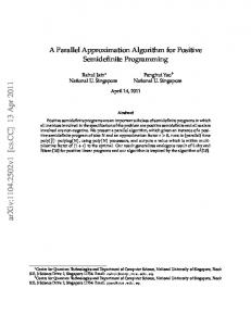
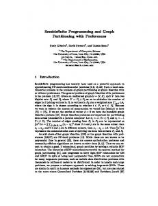
Proof. First we construct a ∈ E(K2,2,2 ) with gd(K2,2,2 , a) ≥ 5, thus implying gd(K2,2,2 ) ≥ 5. For this, let K2,2,2 be obtained from K6 by deleting the edges 5 (1, 4), (2, 5) and (3, 6). Let e1 , . . . , e5 denote the standard unit vectors √ in R , let X be the Gram matrix of the vectors e1 , e2 , e3 , e4 , e5 and (e1 + e2 )/ 2 labeling the nodes 1, . . . , 6, respectively, and let a ∈ E(K2,2,2 ) be the projection of X. We now verify that X is the unique psd completion of a which shows that gd(K2,2,2 , a) ≥ 5. Indeed the chosen Gram labeling of the√matrix X implies the following linear dependency: X[·, 6] = (X[·, 4] + X[·, 5])/ 2 among its columns X[·, i] indexed respectively by i = 4, 5, 6; this implies that the unspecified entries X14 , X25 , X36 are uniquely determined in terms of the specified entries of X. On the other hand, one can easily verify that K2,2,2 is a partial 4-tree, therefore gd(K2,2,2 ) ≤ 5. Moreover, deleting or contracting an edge in K2,2,2 yields a partial 3-tree, thus with Gram dimension at most 4. t u By Lemma 3, all graphs with tree-width at most three belong to G4 . Moreover, these graphs can be characterized in terms of forbidden minors as follows: Theorem 2. [3] A graph G has tw(G) ≤ 3 if and only if G does not have K5 , K2,2,2 , V8 and C5 × C2 as a minor. The graphs V8 and C5 × C2 are shown in Figures 1 and 2 below, respectively. These four graphs are natural candidates for being forbidden minors for the class G4 . We have already seen that for K5 and K2,2,2 this is indeed the case. However, this is not true for V8 and C5 × C2 . Both belong to G4 , this will be proved in Section 3.4 for V8 (Theorem 10) and in Section 4 for C5 × C2 (Theorem 11). These two results form the main technical part of the paper. Using them, we can complete our characterization of the class G4 . Theorem 3. For a graph G, gd(G) ≤ 4 if and only if G does not have K5 or K2,2,2 as a minor. Proof. Necessity follows from Lemmas 1 and 4. Sufficiency follows from the following graph theoretical result, obtained by combining Theorem 2 with Seymour’s splitter theorem (for a self-contained proof see [20]): every graph with no K5 and K2,2,2 minors can be obtained as a subgraph of a clique k-sum (k ≤ 2) of copies of graphs with tree-width at most 3, V8 and C5 × C2 . Combining this fact with Theorems 10, 11 and Lemmas 2, 3 the claim follows. t u 2.3

Links to Euclidean graph realizations

In this section we investigate the links between the Gram dimension and the notion of k-realizability of graphs introduced in [8,9]. We start the discussion with some necessary definitions. Recall that a matrix D = (dij ) ∈ S n is a Euclidean distance matrix (EDM) if there exist vectors p1 , . . . , pn ∈ Rk (for some k ≥ 1) such that dij = kpi − pj k2 for all i, j ∈ [n]. Then EDMn denotes the cone of all n × n Euclidean distance matrices and, for a graph G = ([n], E), EDM(G) = πE (EDMn ) is the set of G-partial matrices that can be completed to a Euclidean distance matrix.

8

Definition 4. Given a graph G = ([n], E) and d ∈ RE + , a Euclidean (distance) representation of d in Rk consists of a set of vectors p1 , . . . , pn ∈ Rk such that kpi − pj k2 = dij ∀ij ∈ E. Then, ed(G, d) is the smallest integer k for which d has a Euclidean representation in Rk and the graph parameter ed(G) is defined as ed(G) =

max

ed(G, d).

(4)

d∈EDM(G)

In the terminology of [8,9] a graph G satisfying ed(G) ≤ k is called krealizable. It is easy to verify that the graph parameter ed(G) is minor monotone. Hence for any fixed k ≥ 1 the class of graphs satisfying ed(G) ≤ k can be characterized by a finite list of minimal forbidden minors. For k ≤ 2 the only forbidden minor is Kk+2 . Belk and Connelly [8,9] have determined the list of forbidden minors for k = 3. Theorem 4. [8,9] For a graph G, ed(G) ≤ 3 if and only if G does not have K5 and K2,2,2 as minors. The hard part of the proof of [8,9] is to prove sufficiency, i.e., that if a graph G has no K5 and K2,2,2 minors then ed(G) ≤ 3. We will obtain this result as a corollary of our main theorem (cf. Corollary 1). To this end, we have to establish some connections between the graphs parameters ed(G) and gd(G). There is a well known correspondence between psd and EDM completions (for details and references see, e.g., [12]). Namely, for a graph G, let ∇G denote its suspension graph, obtained by adding a new node (the apex node, denoted by 0), E(∇G) , adjacent to all nodes of G. Consider the one-to-one map φ : RV ∪E(G) 7→ R+ E(∇G) V ∪E(G) which maps x ∈ R to d = φ(x) ∈ R+ defined by d0i = xii (i ∈ [n]),

dij = xii + xjj − 2xij (ij ∈ E(G)).

Then the vectors u1 , . . . , un ∈ Rk form a Gram representation of x if and only if the vectors u0 = 0, u1 , . . . , un form a Euclidean representation of d = φ(x) in Rk . This shows: Lemma 5. Let G = (V, E) be a graph. Then, gd(G, x) = ed(∇G, φ(x)) for any x ∈ RV ∪E and thus gd(G) = ed(∇G). For the Gram dimension of a graph one can show the following property: Lemma 6. Consider a graph G = (V = [n], E) and its suspension graph ∇G = ([n] ∪ {0}, E ∪ F ), where F = {(0, i) | i ∈ [n]}. Given x ∈ RE , its 0-extension is the vector y = (x, 0) ∈ RE∪F . If x ∈ S+ (G), then y ∈ S+ (∇G) and gd(∇G, y) = gd(G, x) + 1. Moreover, gd(∇G) = gd(G) + 1.

9

Proof. The first part is clear and implies gd(∇G) ≥ gd(G) + 1. Set k = gd(G); n+1 we show the reverse inequality gd(∇G) ≤ k + 1. For this, let X ∈ S+ , written T αa n in block-form as X = , where A ∈ S+ and the first row/column is a A indexed by the apex node 0 of ∇G. If α = 0 then a = 0, πV E (A) has a Gram representation in Rk and thus πV (∇G)E(∇G) (X) too. Assume now α > 0 and without loss of generality α = 1. Consider the Schur complement Y of X with n respect to the entry α = 1, given by Y = A − aaT . As Y ∈ S+ , there exists n Z ∈ S+ such that rank(Z) ≤ k and πV E (Z) = πV E (Y ). Define the matrix 1 aT 0 0 0 X := + . 0Z a aaT Then, rank(X 0 ) = rank(Z) + 1 ≤ k + 1. Moreover, X 0 and X coincide at all diagonal entries as well as at all entries corresponding to edges of ∇G. This concludes the proof that gd(∇G) ≤ k + 1. t u We do not know whether the analogous property is true for the graph parameter ed(G). On the other hand, the following partial result holds, whose proof was communicated to us by A. Schrijver. Theorem 5. For a graph G, ed(∇G) ≥ ed(G) + 1. Proof. Set ed(∇G) = k; we show ed(G) ≤ k − 1. We may assume that G is connected (else deal with each connected component separately). Let d ∈ EDM(G) and let p1 = 0, p2 , . . . , pn be a Euclidean representation of d in Rh (h ≥ 1). Extend the pi ’s to vectors pbi = (pi , 0) ∈ Rh+1 by appending an extra coordinate equal to zero, and set pb0 (t) = (0, t) ∈ Rh+1 where t is any positive real b ∈ EDM(∇G) with Euclidean representascalar. Now consider the distance d(t) tion pb0 (t), pb1 , . . . , pc n. b by As ed(∇G) = k, there exists another Euclidean representation of d(t) k vectors q0 (t), q1 (t), . . . , qn (t) lying in R . Without loss of generality, we can assume that q0 (t) = pb0 (t) = (0, t) and q1 (t) is the zero vector; for i ∈ [n], write qi (t) = (ui (t), ai (t)), where ui (t) ∈ Rk−1 and ai (t) ∈ R. Then kqi (t)k = kpbi k = kpi k whenever node i is adjacent to node 1 in G. As the graph G is connected, this implies that, for any i ∈ [n], the scalars kqi (t)k (t ∈ R+ ) are bounded. Therefore there exists a sequence tm ∈ R+ (m ∈ N) converging to +∞ and for which the sequence (qi (tm ))m has a limit. Say qi (tm ) = (ai (tm ), ui (tm )) converges to (ui , ai ) ∈ Rk as m → +∞, where ui ∈ Rk−1 and ai ∈ R. The condition b 0i implies that kpi k2 + t2 = kui (t)k2 + (ai (t) − t)2 and thus kq0 (t) − qi (t)k2 = d(t) ai (tm ) =

a2i (tm ) + kui (tm )k2 − kpi k2 ∀m ∈ N. 2tm

Taking the limit as m → ∞ we obtain that lim ai (tm ) = 0 and thus ai = 0. m→∞

b m )ij = k(ai (tm ), ui (tm )) − (aj (tm ), uj (tm ))k2 and Then, for i, j ∈ [n], dij = d(t taking the limit as m → +∞ we obtain that dij = kui − uj k2 . This shows that the vectors u1 , . . . , un form a Euclidean representation of d in Rk−1 . t u

10

Combining Lemma 5 with Theorem 5 we obtain the following inequality relating the parameters ed(G) and gd(G). Theorem 6. For any graph G we have that ed(G) ≤ gd(G) − 1. Combining Theorem 6 with our main theorem we can recover sufficiency in Theorem 4. Corollary 1. For a graph G, if G has no K5 and K2,2,2 minors then ed(G) ≤ 3. 2.4

Relation with the graph parameter ν = (G)

In this section we investigate the relation between the Gram dimension of a graph and the graph parameter ν = (G) introduced in [20,21]. Recall that the corank of a matrix M ∈ Rn×n is the dimension of its kernel. Consider the cone n C(G) = {M ∈ S+ : Mij = 0 for all distinct i, j ∈ V with (i, j) 6∈ E}

which, as is well known, can be seen as the dual cone of the cone S+ (G). We now introduce the graph parameter ν = (G). Definition 5. Given a graph G = ([n], E) the parameter ν = (G) is defined as the maximum corank of a matrix M ∈ C(G) satisfying the following property: ∀X ∈ S n

M X = 0, Xii = 0 ∀i ∈ V, Xij = 0 ∀(i, j) ∈ E =⇒ X = 0,

known as the strong Arnold property. It is proven in [20,21] that ν = (G) is a minor monotone graph parameter. Hence for any fixed integer k ≥ 1 the class of graphs with ν = (G) ≤ k can be characterized by a finite family of minimal forbidden minors. For k ≤ 3 the only forbidden minor is Kk+1 . Van der Holst [20,21] has determined the list of forbidden minors for k = 4. Theorem 7. [20,21] For a graph G, ν = (G) ≤ 4 if and only if G does not have K5 and K2,2,2 as minors. By relating the two parameters gd(G) and ν = (G) we can derive sufficiency in Theorem 7 from our main Theorem. Theorem 8. For any graph G, gd(G) ≥ ν = (G). n Proof. Let k = ν = (G) be attained by some matrix M ∈ S+ . Write M = Pn T λ v v , where λ ≥ 0, {v , . . . , v } is an orthonormal base of eigenvectors of i i i 1 n i i=1 Pk M , and {v1 , . . . , vk } spans the kernel of M . Consider the matrix X = i=1 vi viT and its projection a = πE∪V (X) ∈ S+ (G). By construction, rank(X) = k. Hence it is enough to show that a has a unique psd completion, which will imply gd(G) ≥ gd(G, a) = k.

11 n For this let Y ∈ S+ be another psd completion of a. Hence the matrix X − Y has zero entries at all positions (i, j) ∈ V ∪ E. Since the matrix M has zero entries at all off-diagonal positions corresponding to P non-edges of G, we k deduce that hM, X − Y i = 0. On the other hand, hM, Xi = i=1 λi viT M vi = 0. Therefore, hM, Y i = 0. As M, X, Y are psd, the conditions hM, Xi = hM, Y i = 0 imply that M X = M Y = 0 and thus M (X − Y ) = 0. Now we can apply the assumption that the matrix M satisfies the strong Arnold property and deduce that X = Y . t u

Combining Theorem 8 with our main theorem we can recover sufficiency in Theorem 7. Corollary 2. For a graph G, if G does not have K5 and K2,2,2 as minors then ν = (G) ≤ 4. Colin de Verdi`ere [11] studies the graph parameter ν(G), defined as the maximum corank of a matrix M satisfying the strong Arnold property and such that, for any i, j ∈ V , Mij = 0 ⇐⇒ (i, j) 6∈ E. In particular he shows that ν(G) is unbounded for the class of planar graphs. As ν(G) ≤ ν = (G) ≤ gd(G), we obtain as a direct application: Corollary 3. The graph parameter gd(G) is unbounded for the class of planar graphs.

3

Bounding the Gram dimension

In this section we sketch our approach to show that gd(V8 ) = gd(C5 × C2 ) = 4. Definition 6. Given a graph G = (V = [n], E), a configuration of G is an assignment of vectors p1 , . . . , pn (in some space) to the nodes of G; the pair (G, p) is called a framework. We use the notation p = {p1 , . . . , pn } and, for a subset T ⊆ V , pT = {pi | i ∈ T }. Thus p = pV and we also set p−i = pV \{i} . Two configurations p, q of G (not necessarily lying in the same space) are said to be equivalent if pTi pj = qiT qj for all ij ∈ V ∪ E. Our objective is to show that the two graphs G = V8 , C5 × C2 belong to G4 . That is, we must show that, given any a ∈ S+ (G), one can construct a Gram representation q of (G, a) lying in the space R4 . Along the lines of [8] (which deals with Euclidean distance realizations), our strategy to achieve this is as follows: First, we construct a ‘flat’ Gram representation p of (G, a) obtained by maximizing the inner product pTi0 pj0 along a given pair (i0 , j0 ) which is not an edge of G. As suggested in [31] (in the context of Euclidean distance realizations), this configuration p can be obtained by solving a semidefinite program; then p corresponds to the Gram representation of an optimal solution X to this program. In general we cannot yet claim that p lies in R4 . However, we can derive useful information about p by using an optimal solution Ω (which will correspond

12

to a ‘stress matrix’) to the dual semidefinite program. Indeed, the optimality condition XΩ = 0 will imply some linear dependencies among the pi ’s that can be used to show the existence of an equivalent representation q of (G, a) in low dimension. Roughly speaking, most often, these dependencies will force the majority of the pi ’s to lie in R4 , and one will be able to rotate each remaining vector pj about the space spanned by the vectors labeling the neighbors of j into R4 . Showing that the initial representation p can indeed be ‘folded’ into R4 as just described makes up the main body of the proof. Before going into the details of the proof, we indicate some additional genericity assumptions that can be made w.l.o.g. on the vector a ∈ S+ (G). This will be particularly useful when treating the graph C5 × C2 . 3.1

Genericity assumptions

By definition, gd(G) is the maximum value of gd(G, a) taken over all a ∈ E(G). Clearly we can restrict the maximum to be taken over all a lying in a dense subset of E(G). For instance, the set D consisting of all x ∈ E(G) that admit a positive definite completion in En is dense in E(G). We next identify a smaller dense subset D∗ of D which will we use in our study of the Gram dimension of C5 × C2 . We start with a useful lemma, which characterizes the vectors a ∈ E(Cn ) admitting a Gram realization in R2 . Here Cn denotes the cycle on n nodes. Lemma 7. Consider the vector a = (cos ϑ1 , cos ϑ2 , . . . , cos ϑn ) ∈ RE(Cn ) , where n ϑ1 , . . . , ϑn ∈ [0, π]. PnThen gd(Cn , a) ≤ 2 if and only if there exist ∈ {±1} and k ∈ Z such that i=1 i ϑi = 2kπ. Proof. We prove the ‘only if’ part. Assume that u1 , . . . , un ∈ R2 are unit vectors such that uTi ui+1 = cos ϑi for all i ∈ [n] (setting un+1 = u1 ). We may assume that u1 = (1, 0)T . Then, uT1 u2 = cos ϑ1 implies that u2 = (cos(1 ϑ1 ), sin(1 ϑ1 ))T for some 1 ∈ {±1}. Analogously, uT2 u3 = cos ϑ2 implies u3 = (cos(1 ϑ1 + 2 ϑ2 ), sin(1 ϑ1 + 2 ϑ2 ))T for some 2 ∈ {±1}. Iterating, we find that there exists Pi−1 Pi−1 ∈ {±1}n such that ui = (cos( j=1 i ϑi ), sin( j=1 i ϑi ))T for i = 1, . . . , n. Pn−1 Pn Finally, the condition uTn u1 = cos ϑn = cos( i=1 i ϑi ) implies i=1 i ϑi ∈ 2πZ. The arguments can be reversed to show the ‘if part’. t u Lemma 8. Let D∗ be the set of all a ∈ E(G) that admit a positive definite completion in En satisfying the following condition: For any circuit C in G, the restriction aC = (ae )e∈C of a to C does not admit a Gram representation in R2 . Then the set D∗ is dense in E(G). Proof. We show that D∗ is dense in D. Let a ∈ D and set a = cos ϑ, where ϑ ∈ [0, π]E . Given a circuit C in G (say of length p),Pit follows from Lemma 7 p that aC has a Gram realization in R2 if and only if i=1 i ϑi = 2kπ for some p ∈ {±1} and k ∈ Z with |k| ≤ p/2. Let HC denote the union of the hyperplanes in RE(C) defined by these equations. Therefore, a 6∈ D∗ if and only if ϑ ∈ ∪C HC , where the union is taken over all circuits C of G. Clearly we can find a sequence

13

ϑ(i) ∈ [0, π]E \ ∪C HC converging to ϑ as i → ∞. Then the sequence a(i) := cos ϑ(i) tends to a as i → ∞ and, for all i large enough, a(i) ∈ D∗ . This shows that D∗ is a dense subset of D and thus of E(G). t u Corollary 4. For any graph G = ([n], E), gd(G) = max gd(G, a), where the maximum is over all a ∈ E(G) admitting a positive definite completion and whose restriction to any circuit of G has no Gram representation in the plane. 3.2

Semidefinite programming formulation

We now describe how to model the ‘flattening’ procedure using semidefinite programming (sdp) and how to obtain a ‘stress matrix’ using sdp duality. Let G = (V = [n], E) be a graph and let e0 = (i0 , j0 ) be a non-edge of G (i.e., i0 6= j0 and e0 6∈ E). Let a ∈ S+ (G) be a partial positive semidefinite matrix for which we want to show the existence of a Gram representation in a small dimensional space. For this consider the semidefinite program: max hEi0 j0 , Xi s.t. hEij , Xi = aij (ij ∈ V ∪ E), X 0,

(5)

where Eij = (ei eTj + ej eTi )/2 and e1 , . . . , en are the standard unit vectors in Rn . The dual semidefinite program of (5) reads: X X min wij aij s.t. Ω = wij Eij − Ei0 j0 0. (6) ij∈V ∪E

ij∈V ∪E

Theorem 9. Consider a graph G = ([n], E), a pair e0 = (i0 , j0 ) 6∈ E, and let a ∈ S++ (G). Then there exists a Gram realization p = (p1 , . . . , pn ) in Rk (for n satisfying some k ≥ 1) of (G, a) and a matrix Ω = (wij ) ∈ S+ wi0 j0 6= 0,

(7)

wij = 0 for all ij 6∈ V ∪ E ∪ {e0 }, X wii pi + wij pj = 0 for all i ∈ [n],

(8) (9)

j|ij∈E∪{e0 }

dimhpi , pj i = 2 for all ij ∈ E.

(10)

We refer to equation (9) as the equilibrium condition at vertex i. Proof. Consider the sdp (5) and its dual program (6). By assumption, a has a positive definite completion, hence the program (5) is strictly feasible. Clearly, the dual program (6) is also strictly feasible. Hence there is no duality gap and the optimal values are attained in both programs. Let (X, Ω) be a pair of primal-dual optimal solutions. Then (X, Ω) satisfies the optimality condition: hX, Ωi = 0 or, equivalently, XΩ = 0. Say X has rank k and let p = {p1 , . . . , pn } ⊆ Rk be a Gram realization of X. Now it suffices to observe that the condition XΩ = 0 can be reformulated as the equilibrium conditions (9). The conditions (7) and (8) follow from the form of the dual program (6), and (10) follows from the assumption a ∈ S++ (G). t u

14

Note that, using the following variant of Farkas’ lemma for semidefinite programming, one can show the existence of a nonzero positive semidefinite matrix Ω = (wij ) satisfying (8) and the equilibrium conditions (9) also in the case when the sdp (5) is not strictly feasible, however now with wi0 j0 = 0. This remark will be useful in the exceptional case considered in Section 4.5 where we will have to solve again a semidefinite program of the form (5); however this program will have additional conditions imposing that some of the pi ’s are pinned so that one cannot anymore assume strict feasibility (see the proof of Lemma 20). Lemma 9. (Farkas’ lemma for semidefinite programming) (see [28]) Let b ∈ Rm and let A1 , . . . , Am ∈ S n be given. Then exactly one of the following two assertions holds: n (i) Either there exists X ∈ S++ such that hAj , Xi =P bj for j = 1, . . . , m. m (ii) Or there exists a vector y ∈ Rm such that Ω := j=1 yj Aj 0, Ω 6= 0 and T b y ≤ 0.

Moreover, for any X 0 satisfying hAj , Xi = bj (j = 1, . . . , m), we have in (ii) hX, Ωi = bT y = 0 and thus XΩ = 0. Proof. Clearly, if (i) holds then (ii) does not hold. Conversely, assume (i) does n not hold, i.e., S++ ∩ L = ∅, where L = {X ∈ S n | hAj , Xi = bj ∀j}. Then there exists a separating hyperplane, i.e., there exists a nonzero matrix Ω ∈ S n and n and hΩ, Xi ≤ α for all X ∈ L. This α ∈ R such that hΩ, Xi ≥ α for all X ∈ S++ ⊥ implies Ω 0, Ω ∈ L , and α ≤ 0, so that (ii) holds and the lemma follows. t u 3.3

Useful lemmas

We start with some definitions about stressed frameworks and then we establish some basic tools that we will repeatedly use later in our proof for V8 and C5 ×C2 . For a matrix Ω ∈ S n its support graph is the graph S(Ω) is the graph with node set [n] and with edges the pairs (i, j) with Ωij 6= 0. Definition 7. (Stressed framework (H, p, Ω)) Consider a framework (H = (V = [n], F ), p). A nonzero matrix Ω = (wij ) ∈ S n is called a stress matrix for the framework (H, p) if its support graph S(Ω) is contained in H (i.e., wij = 0 for all ij 6∈ V ∪ F ) and Ω satisfies the equilibrium condition X wii pi + wij pj = 0 ∀i ∈ V. (11) j:(i,j)∈F

Then the triple (H, p, Ω) is called a stressed framework, and a psd stressed framework if moreover Ω 0. We let VΩ denote the set of nodes i ∈ V for which Ωij 6= 0 for some j ∈ V . A node i ∈ V is said to be a 0-node when wij = 0 for all j ∈ V . Hence, V \ VΩ is the set of all 0-nodes and, when Ω 0, i is a 0-node if and only if wii = 0. The support graph S(Ω) of Ω is called the stressed graph; its edges are called the stressed edges of H and the nodes i ∈ VΩ are called the stressed nodes. Given an integer t ≥ 1, a node i ∈ V is said to be a t-node if its degree in the stressed graph S(Ω) is equal to t.

15

Throughout we will deal with stressed frameworks (H, p, Ω) obtained by applying Theorem 9. Hence the graph H arises by adding a new edge e0 to a b as indicated below. given graph G, which we then denote as H = G, b Given a graph G = (V = [n], E) and a Definition 8. (Extended graph G) b = (V, E b = E ∪ {e0 }). fixed pair e0 = (i0 , j0 ) not belonging to E, we set G We now group some useful lemmas which we will use in order to show that a given framework (H, p) admits an equivalent configuration in lower dimension. Clearly, the stress matrix provides some linear dependencies among the vectors pi labeling the stressed nodes, but it gives no information about the vectors labeling the 0-nodes. However, if we have a set S of 0-nodes forming a stable set, then we can use the following lemma in order to ‘fold’ the corresponding vectors pi (i ∈ S) in a lower dimensional space. Lemma 10. (Folding the vectors labeling a stable set) Let (H = (V, F ), p) be a framework and let T ⊆ V . Assume that S = V \ T is a stable set in H, that each node i ∈ S has degree at most k − 1 in H, and that dimhpT i ≤ k. Then there exists a configuration q of H in Rk which is equivalent to (H, p). Proof. Fix a node i ∈ S. Let N [i] denote the closed neighborhood of i in H consisting of i and the nodes adjacent to i. By assumption, |N [i]| ≤ k and both sets of vectors pT and pN [i] have rank at most k. Hence one can find an orthogonal matrix P mapping all vectors pj (j ∈ T ∪ N [i]) into the space Rk . Repeat this construction with every other node of S. As no two nodes of S are adjacent, this produces a configuration q in Rk which is equivalent to (H, p). t u The next lemma uses the stress matrix to upper bound the dimension of a given stressed configuration. Lemma 11. (Bounding the dimension) Let (H = (V = [n], F ), p, Ω) be a psd stressed framework. Then dimhpV i ≤ n − 2, except dimhpV i ≤ n − 1 if S(Ω) is a clique. Proof. Let X denote the Gram matrix of the pi ’s, so that rank(X) = dimhpV i. By assumption, XΩ = 0. This implies that rank(X) ≤ n − 1. Moreover, if S(Ω) is not a clique, then rank(Ω) ≥ 2 and thus rank(X) ≤ n − 2. t u The next lemma indicates how 1-nodes can occur in a stressed framework. Lemma 12. Let (H = (V, F ), p, Ω) be a stressed framework. If node i is a 1node in the stressed graph S(Ω), i.e., there is a unique edge ij ∈ F such that wij 6= 0, then dimhpi , pj i ≤ 1. Proof. Directly, using the equilibrium condition (11) at node i.

t u

We now consider 2-nodes in a stressed framework. First recall the notion of Schur complement. For a matrix Ω = (wij ) ∈ S n and i ∈ [n] with wii 6= 0, the Schur complement of Ω with respect to its (i, i)-entry is the matrix, denoted 0 0 as Ω−i = (wjk )j,k∈[n]\{i} ∈ S n−1 , with entries wjk = wjk − wik wjk /wii for i, j ∈ [n] \ {i}. As is well known, Ω 0 if and only if wii > 0 and Ω−i 0. We also need the following notion of ‘contracting a degree two node’ in a graph.

16

Definition 9. Let H = (V, F ) be a graph, let i ∈ V be a node of degree two in H which is adjacent to nodes i1 , i2 ∈ V . The graph obtained by contracting node i in H is the graph H/i with node set V \ {i} and with edge set F/i = F \ {(i, i1 ), (i, i2 )} ∪ {(i1 , i2 )} (ignoring multiple edges). Lemma 13. (Contracting a 2-node) Let (H = (V, F ), p, Ω) be a psd stressed framework, let i ∈ V be a 2-node in the stressed graph S(Ω) and set N (i) = {i1 , i2 }. Then pi ∈ hpi1 , pi2 i and thus dimhpi = dimhp−i i. Moreover, if the stressed graph S(Ω) is not the complete graph on N [i] = {i, i1 , i2 }, then (H/i, p−i , Ω−i ) is a psd stressed framework. Proof. The equilibrium condition at node i implies pi ∈ hpi1 , pi2 i. Note that the Schur complement Ω−i of Ω with respect to the (i, i)-entry wii has entries 0 2 /wii for r = 1, 2, and wjk = wjk wi01 i2 = wi1 i2 − wii1 wii2 /wii , wi0r ir = wir ir − wii r for all other edges jk of H/i. As Ω 0 we also have Ω−i 0. Moreover, Ω−i 6= 0. Indeed, wi01 i2 6= 0 if (i1 , i2 ) 6∈ F ; otherwise, as S(Ω) is not the clique on N [i], 0 there is another edge jk of H/i in the support of Ω so that wjk = wjk 6= 0. In order to show that Ω−i is a stress matrix for (H/i, p−i ), it suffices to check the stress equilibrium at the nodes i1Pand i2 . To fix ideas consider P node i1 . Then we can rewrite wi01 i1 pi1 + wi01 i2 pi2 + j∈N (i1 )\{i2 } wi01 j pj as ( j wi1 j pj ) − (wii pi + wii1 pi1 + wii2 pi2 ) wii1 /wii , where both terms are equal to 0 using the equilibrium conditions of (Ω, p) at nodes i1 and i. t u We will apply the above lemma iteratively to contract a set I containing several 2-nodes. Of course, in order to obtain useful information, we want to be able to claim that, after contraction, we obtain a stressed framework (H/I, pV \I , Ω−I ), i.e., with Ω−I 6= 0. Problems might occur if at some step we get a stressed graph which is a clique on 3 nodes. Note that this can happen only when a connected component of the stressed graph is a circuit. However, when we will apply this operation of contracting 2-nodes to the case of G = C5 × C2 , we will make sure that this situation cannot happen; that is, we will show that we may assume that the stressed graph does not have a connected component which is a circuit (see Remark 1 in Section 4.1). 3.4

The graph V8 has Gram dimension 4

Let V8 = (V = [8], E) be the graph shown in Figure 1. In this section we use the tools developed above to show that V8 has Gram dimension 4. Theorem 10. The graph V8 has Gram dimension 4. Proof. Set G = V8 = ([8], E). Clearly gd(G) ≥ 4 since K4 is a minor of G. Fix a ∈ S++ (G); we show that (G, a) has a Gram realization in R4 . For this we first apply Theorem 9. As stretched edge e0 , we choose the pair e0 = (1, 4) and we b = ([8], E b = E ∪ {(1, 4)}) the extended graph obtained by adding denote by G the stretched pair (1, 4) to G. Let p be the initial Gram realization of (G, a) and let Ω = (wij ) be the corresponding stress matrix obtained by applying Theorem

17

5

6

4

7

3

8

2

1

Fig. 1. The graph V8 .

9. We now show how to construct from p an equivalent realization q of (G, a) lying in R4 . In view of Lemma 10, we know that we are done if we can find a subset S ⊆ V which is stable in the graph G and satisfies dimhpV \S i ≤ 4. This permits to deal with 1-nodes. Indeed suppose that there is a 1-node in the stressed graph S(Ω). In view of Lemma 12 and (10), this can only be node 1 (or node 4) (i.e., the end points of the stretched pair) and dimhp1 , p4 i ≤ 1. Then, choosing the stable set S = {2, 5, 7}, we have dimhpV \S i ≤ 4 and we can conclude using Lemma 10. Hence we can now assume that there is no 1-node in the stressed graph S(Ω). Next, observe that we are done in any of the following two cases: (i) There exists a set T ⊆ V with |T | = 4 and dimhpT i ≤ 2. (ii) There exists a set T ⊆ V of cardinality |T | = 3 such that T does not consist of three consecutive nodes on the circuit (1, 2, . . . , 8) and dimhpT i ≤ 2. Indeed, in case (i) (resp., case (ii)), there is a stable set S ⊆ V \ T of cardinality |S| = 2 (resp., |S| = 3), so that |V \ (S ∪ T )| = 2 and thus dimhpV \S i ≤ dimhpT i + dimhpV \(S∪T ) i ≤ 2 + 2 = 4. Hence we may assume that we are not in the situation of cases (i) and (ii). Assume first that one of the nodes in {5, 6, 7, 8} is a 0-node. Then all of them are 0-nodes. Indeed, if (say) 5 is a 0-node and 6 is not a 0-node then the equilibrium equation at node 6 implies that dimhp6 , p7 , p2 i ≤ 2 so that we are in the situation of case (ii). As nodes 1, 4 are not 1-nodes, the stressed graph S(Ω) is the circuit (1, 2, 3, 4). Using Lemma 13, we deduce that dimhp1 , p2 , p3 , p4 i ≤ 2 and thus we are in the situation of case (i) above. Assume now that none of the nodes in {5, 6, 7, 8} is a 0-node but one of the nodes in {2, 3} is a 0-node. Then both nodes 2 and 3 are 0-nodes (else we are in the situation of case (ii)). Therefore, both nodes 6 and 7 are 2-nodes. Applying Lemma 13, after contracting both nodes 6,7, we obtain a stressed framework on {1, 4, 5, 8} and thus dimhpV \{2,3} i = dimhp1 , p4 , p5 , p8 i. Using Lemma 11, we deduce that dimhp1 , p4 , p5 , p8 i ≤ 3. Therefore, dimhpV \{3} i ≤ 4 and one can find a new realization q in R4 equivalent to (G, p) using Lemma 10.

18

Finally assume that none of the nodes in {2, 3, 5, 6, 7, 8} is a 0-node. We show that hpi = hp2 , p3 , p6 , p7 i. The equilibrium equation at node 6 implies that dimhp2 , p5 , p6 , p7 i ≤ 3. Moreover, dimhp2 , p6 , p7 i = 3 (else we are in case (ii) above). Hence p5 ∈ hp2 , p6 , p7 i. Analogously, the equilibrium equations at nodes 7,2,3 give that p8 , p1 , p4 ∈ hp2 , p3 , p6 , p7 i, respectively. t u

4

The graph C5 × C2 has Gram dimension 4

This section is devoted to proving that the graph C5 × C2 has Gram dimension 4. The analysis is considerably more involved than the analysis for V8 . Figure 2 shows two drawings of C5 × C2 , the second one making its symmetries more apparent. Theorem 11. The graph C5 × C2 has Gram dimension 4. Throughout this section we set G = C5 × C2 = (V = [10], E). Clearly, gd(G) ≥ 4 since K4 is a minor of G. In order to show that gd(G) ≤ 4, we must show that gd(G, a) ≤ 4 for any a ∈ S++ (G). Moreover, in view of Corollary 4, it suffices to show this for all a ∈ S++ (G) satisfying the following ‘genericity’ property: For any Gram realization p of (G, a), dimhpC i ≥ 3 for any circuit C in G.

(12)

From now on, we fix a ∈ S++ (G) satisfying this genericity property. Our objective is to show that there exists a Gram realization of (G, a) in R4 . Again we use Theorem 9 to construct an initial Gram realization p of (G, a). b = As stretched edge e0 , we choose the pair e0 = (3, 8) and we denote by G b ([8], E = E ∪ {(3, 8)}) the extended graph obtained by adding the stretched pair b p, Ω) is a (3, 8) to G. By Theorem 9, we also have a stress matrix Ω so that (G, psd stressed framework. Our objective is now to construct from p another Gram realization q of (G, a) lying in R4 . 4.1

Additional useful lemmas

First we deal with the case when dimhpi , pj i = 1 for some pair (i, j) of distinct nodes. As a ∈ S++ (G), this can only happen when (i, j) 6∈ E. Lemma 14. If dimhpi , pj i = 1 for some pair (i, j) 6∈ E, then there is a configuration in R4 equivalent to (G, p). Proof. By assumption, pi = pj for some scalar 6= 0. Up to symmetry there are two cases to consider: (i) (i, j) = (1, 5) (two nodes at distance 2 in G), or (ii) (i, j) = (1, 6) (two nodes at distance 3). Consider first case (i) when (i, j) = (1, 5), so p1 = p5 . Set V 0 = V \ {1}. Let G0 = (V 0 , E 0 ) be the graph on V 0 obtained from G by deleting node 1 and adding the edges (2, 5) and (5, 9) (in other words, get G0 by identifying nodes 1 and 5 in G). Let X 0 be the Gram matrix of the

19

7

3 2

4

8 5

6

10 4

2

1

5

10

6

9

9 3

1

7 8

Fig. 2. Two drawings of the graph C5 × C2 .

0 vectors pi (i ∈ V 0 ) and define a0 = (Xjk )jk∈V 0 ∪E 0 ∈ S+ (G0 ). First we show that 0 0 4 (G , a ) has a Gram realization in R . For this, consider the graph H obtained from G by deleting both nodes 1 and 5. Then G0 is a subgraph of ∇H and thus gd(G0 ) ≤ gd(∇H) = gd(H) + 1. As tw(H) ≤ 2 it follows that gd(H) ≤ 3 and thus gd(G0 ) ≤ 4. Finally, if qV 0 is a Gram realization in R4 of (G0 , a0 ) then, setting q1 = q5 , we obtain a Gram realization q of (G, a) in R4 . Case (ii) is analogous, based on the fact that the graph H obtained from G by deleting nodes 1 and 6 is a partial 2-tree. t u

We now consider the case when the stressed graph might have a circuit as a connected component. b If C is a connected component of S(Ω), Lemma 15. Let C be a circuit in G. then dimhpC i ≤ 2. Proof. Directy, using Lemma 13 combined with Lemma 11.

t u

Therefore, in view of the genericity assumption (12), if a circuit C is a connected component of the stressed graph, then C cannot be a circuit in G and thus C must contain the stretched pair e0 = (3, 8). The next result is useful to handle this case, treated in Corollary 5 below. Lemma 16. Let N2 (i) be the set of nodes at distance 2 from a given node i in G. If dimhpN2 (i) i ≤ 3, then there is a configuration equivalent to (G, p) in R4 . Proof. Say, i = 1 so that N2 (1) = {4, 5, 7, 10}, cf. Figure 3. Consider the set S = {2, 3, 6, 9} which is stable in G. Let H denote the graph obtained from G in the following way: For each node i ∈ S, delete i and add the clique on N (i). One can verify that H is contained in the clique 4-sum of the two cliques H1 and H2 on the node sets V1 = {1, 4, 5, 7, 10} and V2 = {4, 5, 7, 8, 10}, respectively. By assumption, dimhpV1 i ≤ 4 and dimhpV2 i ≤ 4. Therefore, one can apply an orthogonal transformation and find vectors qi ∈ R4 (i ∈ V1 ∪ V2 ) such that pVr and qVr have the same Gram matrix, for r = 1, 2. Finally, as V1 ∪ V2 = V \ S

20

and the set S is stable in G, one can extend to a configuration qV equivalent to pV by applying Lemma 10. t u b containing the (stretched) edge (3, 8) Corollary 5. If there is a circuit C in G such that dimhpC i ≤ 2, then there is a configuration equivalent to (G, p) in R4 . Proof. If |C| ≥ 7, pick i ∈ V \ C and note that dimhp−i i ≤ 4. If |C| = 6, pick a subset S ⊆ V \ C of cardinality 2 which is stable in G, so that dimhpV \S i ≤ 4. In both cases we can conclude using Lemma 10. Assume now that |C| = 4 or 5. In view of Lemma 16, it suffices to check that there exists a node i for which |C ∩ N2 (i)| = 3. For instance, for C = (3, 8, 7, 5), this holds for node i = 9, and for C = (3, 8, 10, 9, 1) this holds for i = 2. Then, Lemma 16 implies that dimhpN2 (i) i ≤ 3. t u Remark 1. From now on, we will assume that dimhpi , pj i = 2 for all i 6= j ∈ V (by Lemma 14). Hence there is no 1-node in the stressed graph. Moreover, we b satisfies dimhpC i ≤ 2. Therefore, the stressed will assume that no circuit C of G graph does not have a connected component which is a circuit (by (12), Lemma 15 and Corollary 5). Hence we are guaranteed that after contracting several 2-nodes we do obtain a stressed framework (i.e, with a nonzero stress matrix). The next two lemmas settle the case when there are sufficiently many 2-nodes. Lemma 17. If there are at least four 2-nodes in the stressed graph S(Ω), then there is a configuration equivalent to (G, p) in R4 . Proof. Let I be a set of four 2-nodes in S(Ω). Hence, pI ⊆ hpV \I i and thus it suffices to show that dimhpV \I i ≤ 4. After contracting each of the four 2-nodes of I, we obtain a psd stressed b pV \I , Ω 0 ). Indeed, we can apply Lemma 13 and obtain a nonzero framework (G/I, psd stress matrix Ω 0 in the contracted graph (recall Remark 1). If the support graph of Ω 0 is not a clique, Lemma 11 implies that dimhpV \I i ≤ |V \ I| − 2 = 4. Assume now that S(Ω 0 ) is a clique on T ⊆ V \ I. Then dimhpT i ≤ t − 1, |V \ (I ∪ T )| = 6 − t, and t = |T | ∈ {3, 4, 5}. Indeed one cannot have t = 6 since, after contracting the four 2-nodes, at least 4 edges are lost so that there remains at most 16 − 4 = 12 < 15 edges. It suffices now to show that we can partition V \ (I ∪ T ) as S ∪ S 0 , where S is stable in G and |S 0 | + t − 1 ≤ 4. Indeed, we then have dimhpV \S i = dimhpT ∪S 0 i ≤ t − 1 + |S 0 | ≤ 4 and we can conclude using Lemma 10. If t = 5, then |V \ (I ∪ T )| = 1 and choose S 0 = ∅. If t = 4, then choose S 0 ⊆ V \ (I ∪ T ) of cardinality 1. If t = 3, then one can choose a stable set of cardinality 2 in V \ (I ∪ T ) and |S 0 | = 1. t u Lemma 18. If there is at least one 0-node and at least three 2-nodes in the stressed graph S(Ω), then there is a configuration equivalent to (G, p) in R4 . Proof. For r = 0, 2, let Vr denote the set of r-nodes and set nr = |Vr |. By assumption, n0 ≥ 1 and we can assume n2 = 3 (else apply Lemma 17). Set W = V \ (V0 ∪ V2 ). After contracting the three 2-nodes in the stressed framework

21

b p, Ω), we get a stressed framework (H, pW , Ω 0 ) on |W | = 7−n0 nodes. Hence (G, n0 ≤ 4 and pV2 ⊆ hpW i. Assume first that S(Ω 0 ) is not a clique. Then dimhpW i ≤ |W | − 2 = 5 − n0 by Lemma 11. Now we can conclude using Lemma 10 since in each of the cases: n0 = 1, 2, 3, 4, one can find a stable set S ⊆ V0 such that dimhpW ∪(V0 \S) i ≤ 4. Assume now that S(Ω 0 ) is a clique. Then dimhpW i ≤ |W | − 1 = 6 − n0 by Lemma 11. Note first that n0 6= 1, 2. Indeed, if n0 = 1 then, after deleting the 0-node and contracting the three 2-nodes, we have lost at least 3 + 3 = 6 edges. Hence there remains at most 16 − 6 = 10 edges in the stressed graph S(Ω 0 ), which therefore cannot be a clique on six nodes. If n0 = 2 then, after deleting the two 0-nodes and contracting the three 2-nodes, we have lost at least 5 + 3 = 8 edges. Hence there remain at most 16 − 8 = 8 edges in the stressed graph S(Ω 0 ), which therefore cannot be a clique on five nodes. In each of the two cases n0 = 3, 4, one can find a stable set S ⊆ V0 of cardinality 2 and thus dimhpW ∪(V0 \S) i ≤ (6 − n0 ) + (n0 − 2) = 4. Again conclude using Lemma 10. t u 4.2

Sketch of the proof

In the proof we distinguish two cases: (i) when there is no 0-node, and (ii) when there is at least one 0-node, which are considered, respectively, in Sections 4.3 and 4.4. In both cases the tools developed in the preceding section permit to conclude, except in one exceptional situation, occurring in case (ii). This execptional situation is when nodes 1,2,9 and 10 are 0-nodes and all edges of b \ {1, 2, 9, 10} are stressed. This situation needs a specific treatment which is G done in Section 4.5. 4.3

There is no 0-node in the stressed graph

In this section we consider the case when each node is stressed in S(Ω), i.e., wii 6= 0 for all i ∈ [n]. Lemma 19. Assume that all vertices are stressed in the stressed graph S(Ω) and that there exists a circuit C of length 4 in G such that all edges in the cut b with i ∈ C and j ∈ V \ C. δ(C) are stressed, i.e., wij 6= 0 for all edges ij ∈ E Then dimhpV i ≤ 4. Proof. Up to symmetry, there are three types of circuits C of length 4 to consider: (i) C does not meet {3, 8}, i.e., C = (1, 2, 10, 9); or (ii) C contains one of the two nodes 3,8, say node 8, and it contains a node adjacent to the other one, i.e., node 3, like C = (5, 6, 8, 7); or (iii) C contains one of 3,8 but has no node adjacent to the other one, like C = (7, 8, 10, 9). Consider first the case (i), when C = (1, 2, 10, 9). We show that the set pC spans pV . Using the equilibrium conditions at the nodes 1,2,9,10, we find that p3 , p4 , p7 , p8 ∈ hpC i. As 6 is not a 0-node, w6i 6= 0 for some i ∈ {4, 8}. Then, the equilibrium condition at node i implies that p6 ∈ hpC i. Analogously for node 5.

22

Case (ii) when C = (5, 6, 8, 7) can be treated in analogous manner. Just note that the equilibrium conditions applied to nodes 7,5,6 and 8 respectively, imply that p9 , p3 , p4 , p10 ∈ hpC i. We now consider case (iii) when C = (7, 8, 10, 9). Then one sees directly that p1 , p2 , p5 ∈ hpC i. If w24 6= 0, then the equilibrium conditions at nodes 2,3,6 imply that p4 , p3 , p6 ∈ hpC i and thus hpC i = hpV i. Assume now that w24 = 0, which implies w34 , w46 6= 0. If w13 6= 0, then the equilibrium conditions at nodes 1,3,4 imply that pC spans p3 , p4 , p6 and we are done. Assume now that w24 = w13 = 0, so that 1,2,4 are 2-nodes. If there is one more 2-node then we are done by Lemma 17. Hence we can now assume that wij 6= 0 whenever (i, j) 6= (2, 4) or (1, 3). After b p, Ω), we contracting the three 2-nodes 1,2,4 in the psd stressed framework (G, obtain a new psd stressed framework on V \{1, 2, 4} where nodes 9, 10 have again degree 2. So contract these two nodes and get another psd stressed framework on V \ {1, 2, 4, 9, 10}. Finally this implies dimhpV i = dimhpV \{1,2,4,9,10} i ≤ 4. t u In view of Lemma 19, we can now assume that, for each circuit C of length 4 in G, there is at least one edge ij ∈ δ(C) which is not stressed, i.e., wij = 0. It suffices now to show that this implies the existence of at least four 2-nodes, as we can then conclude using Lemma 17. For this let us enumerate the cuts δ(C) of the 4-circuits C in G: • For C = (1, 2, 10, 9), δ(C) = {(1, 3), (2, 4), (7, 9), (8, 10)}. • For C = (7, 9, 10, 8), δ(C) = {(1, 9), (2, 10), (5, 7), (6, 8)}. • For C = (5, 6, 8, 7), δ(C) = {(7, 9), (8, 10), (3, 5), (4, 6)}. • For C = (3, 5, 6, 4), δ(C) = {(1, 3), (2, 4), (5, 7), (6, 8)}. • For C = (1, 3, 4, 2), δ(C) = {(3, 5), (4, 6), (1, 9), (2, 10)}. For instance, w24 = 0 implies that both 2 and 4 are 2-nodes, while w13 = 0 implies that 1 is a 2-node. One can easily verify that there are at least four 2-nodes in S(Ω). 4.4

There is at least one 0-node in the stressed graph

Note that the mapping σ : V → V that permutes each of the pairs (1, 10), (4, 7), (5, 6), (2, 9) and (3, 8) is an automorphism of G. This can be easily seen using the second drawing of C5 × C2 in Figure 2. Hence, as nodes 3 and 8 are not 0-nodes, up to symmetry, it suffices to consider the following three cases: • Node 1 is a 0-node. • Nodes 1, 10 are not 0-nodes and node 4 is a 0-node. • Nodes 1, 10, 4, 7 are not 0-nodes and one of 5 or 2 is a 0-node. b from Figure 3. Node 1 is a 0-node. It will be useful to use the drawing of G There, the thick edge (3,8) is known to be stressed, the dotted edges are known to be non-stressed (i.e., wij = 0), while the other edges could be stressed or not. In view of Lemma 18, we can assume that there are at most two 2-nodes (else we are done).

23 1

3

2

5

4

6

9

10

7

8

Fig. 3. A drawing of C\ 5 × C2 with 1 as the root node.

Assume first that both nodes 2 and 9 are 0-nodes. Then node 10 too is a 0node and each of nodes 4 and 7 is a 0- or 2-node. If both 4,7 are 2-nodes, then all edges in the graph G\{1, 2, 9, 10} are stressed. Hence we are in the exceptional case, which we will consider in Section 4.5 below. If 4 is a 0-node and 7 is a 2-node, then 3,7 must be the only 2-nodes and thus 6 is a 0-node. Hence, the stressed graph is the circuit C = (3, 8, 5, 7), which implies dimhpC i ≤ 2 and thus we can conclude using Corollary 5. If 4 is a 2-node and 7 is a 0-node, then we find at least two more 2-nodes. Finally, if both 4,7 are 0-nodes, then the stressed graph is the circuit C = (3, 8, 6, 5) and thus we can again conclude using Corollary 5. We can now assume that at least one of the two nodes 2,9 is a 2-node. Then, node 3 has degree 3 in the stressed graph. (Indeed, if 3 is a 2-node, then 10 must be a 0-node (else we have three 2-nodes), which implies that 2,9 are 0nodes, a contradiction.) If exactly one of nodes 2,9 is stressed, one can easily see that there should be at least three 2-nodes. Finally consider the case when both nodes 2,9 are stressed. Then they are the only 2-nodes which implies that all edges of G\1 are stressed. Set I = {4, 5, 8}. We show that pI spans pV \{1} , so that p{1,4,5,8} spans pV . Indeed, the equilibrium conditions at 3 and 6 imply that p3 , p6 ∈ hpI i. Next, the equilibrium conditions at 4, 5, 2, 9 imply, respectively, that p2 ∈ hp3 , p4 , p6 i ⊆ hpI i, p7 ∈ hp3 , p5 , p6 i ⊆ hpI i, p10 ∈ hp2 , p4 i ⊆ hpI i, and p9 ∈ hp7 , p10 i ⊆ hpI i. This concludes the proof. Nodes 1, 10 are not 0-nodes and node 4 is a 0-node. It will be useful to b from Figure 4. We can assume that node 2 is a 2-node and use the drawing of G that node 3 has degree 3 in the stressed graph, since otherwise one would find at least three 2-nodes. Consider first the case when 6 is a 2-node. Then nodes 2 and 6 are the only 2-nodes which implies that all edges in the graph G\4 are stressed. Set I = {3, 5, 7, 10}. We show that pI spans pV \{4} , and then we can conclude using Lemma 10. Indeed, the equilibrium conditions applied, respectively, to nodes 5,6,3,1,2 imply that p6 ∈ hpI i, p8 ∈ hp5 , p6 i ⊆ hpI i, p1 ∈ hp3 , p5 , p8 i ⊆ hpI i, p9 ∈ hp1 , p7 , p10 i ⊆ hpI i, p2 ∈ hp1 , p10 i ⊆ hpI i.

24 4

3

6

8

2

5

1

10

7

9


Consider now the case when 6 is a 0-node. Then 2 and 5 are the only 2nodes so that all edges in the graph G\{4, 6} are stressed. Set I = {3, 7, 10}. We show that pI spans pV \{4,6} , and then we can again conclude using Lemma 10. Indeed the equilibrium conditions applied, respectively, at nodes 5,8,3,2,1 imply that p5 , p8 ∈ hpI i, p1 ∈ hp3 , p5 , p8 i ⊆ hpI i, p2 ∈ hp1 , p10 i ⊆ hpI i, p9 ∈ hp2 , p8 , p10 i ⊆ hpI i. Nodes 1, 4, 7, 10 are not 0-nodes and node 5 or 2 is a 0-node. It will b from Figure 5. We assume that nodes 1,4,7,10 be useful to use the drawing of G are not 0-nodes. Consider first the case when node 5 is a 0-node. Then node 7 is a 2-node. 5

7

6

9

8

10

3

4

1

2


If node 6 is a 2-node, then 6 and 7 are the only 2-nodes and thus all edges of the graph G\5 are stressed. Setting I = {1, 2, 4, 8}, one can verify that pI spans pV \{5} and then one can conclude using Lemma 10.

25

If node 6 is a 0-node, then nodes 4 and 7 are the only 2-nodes and thus all edges in the graph G\{5, 6} are stressed. Setting I = {2, 3, 9}, one can verify that pI spans pV \{5,6} . Thus p{2,3,9,6} spans pV \{5} and one can again conclude using Lemma 10. Consider finally the case when nodes 1,4,7,10, 5 and 6 are not 0-nodes and node 2 is a 0-node. As node 2 is adjacent to nodes 1, 4 and 10 in G, we find three 2-nodes and thus we are done. 4.5

The exceptional case

In this section we consider the following case which was left open in the first case considered in Section 4.4: Nodes 1, 2, 9 and 10 are 0-nodes and all edges of b the graph G\{1, 2, 9, 10} are stressed. Then, nodes 4 and 7 are 2-nodes in the stressed graph. After contracting both nodes 4,7, we obtain a stressed graph which is the complete graph on 4 nodes. Hence, using Lemma 11, we can conclude that dimhpV1 i ≤ 3, where V1 = V \ {1, 2, 9, 10}. Among the nodes 1, 2, 9 and 10, we can find a stable set of size 2. Hence, if dimhpV1 i ≤ 2 then, using Lemma 10, we can find an equivalent configuration in dimension 2 + 2 = 4 and we are done. From now on we assume that dimhpV1 i = 3. (13) In this case it is not clear how to fold p in R4 . In order to settle this case, we proceed as in Belk [8]: We fix (or pin) the vectors pi labeling the nodes i ∈ V1 and we search for another set of vectors p0i labeling the nodes i ∈ V2 = V \ V1 = {1, 2, 9, 10} so that pV1 ∪ p0V2 can be folded into R4 . Again, our starting point is to get such new vectors p0i (i ∈ V2 ) which, together with pV1 , provide a Gram realization of (G, a), by stretching along a second pair e0 ; namely we stretch the pair e0 = (4, 9) ∈ V1 × V2 . As in So and Ye [31], this configuration p0V2 is again obtained by solving a semidefinite program; details are given below. Computing p0V2 via semidefinite programming. Let E[V2 ] denote the set of edges of G contained in V2 and let E[V1 , V2 ] denote the set of edges (i, j) ∈ E with i ∈ V1 , j ∈ V2 . Moreover, set |V1 | = n1 ≥ |V2 | = n2 , so the configuration pV1 lies in Rn1 . (Here n1 = 6, n2 = 4). We now search for a new configuration p0V2 by stretching along the pair (4, 9). For this we use the following semidefinite program: max hF49 , Zi such that hFij , Zi = aij hEij , Zi = aij hEij , Zi = 0 hEii , Zi = 1 Z 0.

∀ij ∈ E[V1 , V2 ] ∀ij ∈ V2 ∪ E[V2 ] ∀i < j, i, j ∈ V1 ∀i ∈ V1

(14)

Here, Eij = (ei eTj + ej eTi )/2 ∈ S n1 +n2 , where ei (i ∈ [n1 + n2 ]) are the standard unit vectors in Rn1 +n2 . Moreover, for i ∈ V1 , j ∈ V2 , Fij = (p0i eTj + ej (p0i )T )/2, after setting p0i = (pi , 0) ∈ Rn1 +n2 .

26

Consider nowa matrix Z feasible for (14). Then Z can be written in the In1 Y block form Z = , and let yi ∈ Rn1 (i ∈ V2 ) denote the columns of Y . YT X The condition Z 0 is equivalent to X − Y T Y 0. Say, X − Y T Y is the Gram matrix of the vectors zi ∈ Rn2 (i ∈ V2 ). For i ∈ V2 , set p0i = (yi , zi ) ∈ Rn1 +n2 . Then X is the Gram matrix of the vectors p0i (i ∈ V2 ). For i ∈ V1 , j ∈ V2 we have that hFij , Zi = (pi , 0)T (yj , zj ) = (p0i )T p0j . Moreover, for i, j ∈ V2 , we have that hEij , Zi = Xij = (p0i )T p0j . Therefore, the linear conditions hFij , Zi = aij for ij ∈ E[V1 , V2 ] and hEij , Zi = aij for ij ∈ V2 ∪ E[V2 ] imply that the vectors p0i (i ∈ V1 ∪ V2 ) form a Gram realization of (G, a). We now consider the dual semidefinite program of (14) which, as we see in Lemma 20 below, will give us some equilibrium conditions on the new vectors 0 p0i (i ∈ V2 ). The dual program involves scalar variables wij (for ij ∈ E[V1 , V2 ] ∪ U 0 V2 ∪ E[V2 ]) and a matrix U 0 = , and it reads: 0 0 min

hIn1 , U i +

X

0 wij aij

ij∈V2 ∪E[V2 ]

ij∈E[V1 ,V2 ]

such that Ω 0 = −F49 + U 0 +

X

0 wij aij +

X

0 wij Fij +

ij∈E[V1 ,V2 ]

X

0 wij Eij 0.

(15)

ij∈V2 ∪E[V2 ]

Since the primal program (14) is bounded and the dual program (15) is strictly feasible it follows that program (14) has an optimal solution Z. Let p0i ∈ Rn1 +n2 (i ∈ V1 ∪ V2 ) be the vectors as defined above, which thus form a Gram realization of (G, a). 0 Lemma 20. There exists a nonzero matrix Ω 0 = (wij ) 0 satisfying the opti0 mality condition ZΩ = 0 and the following conditions on its support: 0 wij = 0 ∀(i, j) ∈ (V1 × V2 ) \ (E[V1 , V2 ] ∪ {(4, 9)}), 0 wij = 0 ∀i 6= j ∈ V2 , (i, j) 6∈ E[V2 ].

Moreover, the following equilibrium conditions hold: X 0 0 0 0 wii pi + wij pj = 0 ∀i ∈ V2

(16)

(17)

j∈V1 ∪V2 |ij∈E∪{(4,9)} 0 and wij 6 0 for some ij ∈ V2 ∪ E[V2 ]. Furthermore, a node i ∈ V2 is a 0-node, = 0 0 i.e., wij = 0 for all j ∈ V1 ∪ V2 , if and only if wii = 0.

Proof. If the primal program (14) is strictly feasible, then (15) has an optimal 0 = −1). Otherwise, if solution Ω 0 which satisfies ZΩ 0 = 0 and (16) (with w49 (14) is feasible but not strictly feasible then, using Farkas’ lemma (Lemma 9), 0 = 0). we again find a matrix Ω 0 0 satisfying ZΩ 0 = 0 and (16) (now with w49 0 We now indicate how to derive (17) from the condition ZΩ = 0.

27

For this write the matrices Z and Ω 0 in block form 0 I Y Ω10 Ω12 Z = nT1 , Ω0 = . 0 T Y X (Ω12 ) Ω20 0 0 From ZΩ 0 = 0, we derive Y T Ω12 + XΩ20 = 0 and Ω12 + Y Ω20 = 0. First this T 0 implies (X − Y Y )Ω2 = 0 which in turn implies that the V2 -coordinates of the vectors on the left hand side in (17) are equal P to 0. Second, the condition 0 0 0 0 T Ω12 + Y Ω20 = 0 together with expressing Ω12 = ij∈E[V1 ,V2 ]∪{(4,9)} wij pi ej , implies that the V1 -coordinates of the vectors on the left hand side in (17) are 0. 0 Thus (17) holds. Finally, we verify that Ω20 6= 0. Indeed, Ω20 = 0 implies Ω12 =0 0 0 0 and thus Ω = 0 since 0 = hZ, Ω i = hIn1 , Ω1 i. t u

Folding p0 into R4 . We now use the above configuration p0 and the equilibrium conditions (17) at the nodes of V2 to construct a Gram realization of (G, a) in R4 . By construction, p0i = (pi , 0) for i ∈ V1 . Note that no node i ∈ V2 is a 1-node with respect to the new stress Ω 0 (recall Lemma 14). Let us point out again 0 that Lemma 20 does not guarantee that w49 6= 0 (as opposed to relation (7) in Theorem 9). By assumption nodes 1,2,9 and 10 are 0-nodes and all other edges of the b \ {1, 2, 9, 10} are stressed w.r.t. the old stress matrix Ω. We begin with graph G the following easy observation about p0V1 . Lemma 21. dimhp04 , p07 , p08 i = dimhp03 , p04 , p08 i = 3. Proof. It is easy to see that each of these sets spans p0V1 and dimhp0V1 i = dimhpV1 i = 3 by (13). t u As an immediate corollary we may assume that p0i 6∈ hp0V1 i ∀i ∈ V2 p0i

hp0V1 i

(18)

Indeed, if there exists i ∈ V2 satisfying ∈ then we can find a stable set of size two in V2 \ {i} and using Lemma 10 we can construct an equivalent configuration in R4 . Therefore, we can assume that at most two nodes in V2 are 0-nodes in S(Ω 0 ) since, by construction, for the new stress matrix Ω 0 there exists 0 ij ∈ V2 ∪ E[V2 ] such that wij 6= 0. This guides our discussion below. Figure 6 shows the graph containing the support of the new stress matrix Ω 0 . There are two 0-nodes in V2 . The cases when either 2,9, or 1,10, are 0-nodes are excluded (since then one would have a 1-node). If nodes 1 and 9 are 0-nodes, then the equilibrium conditions at nodes 2 and 10 imply that p04 , p08 ∈ hp02 , p010 i and by Lemma 21 we have that hp02 , p010 i = hp04 , p08 i ⊆ hp0V1 i, contradicting (18). The case when nodes 9,10 are 0-nodes is similar. Finally assume that nodes 1,2 are 0-nodes (the case when 2,10 are 0-nodes 0 is analogous). As w8,10 6= 0, the equilibrium condition at node 10 implies that 0 0 0 0 p8 ∈ hp9 , p10 i. If w49 = 0 then the equilibrium condition at node 9 implies that p07 ∈ hp09 , p010 i. Hence hp07 , p08 i ⊆ hp09 , p010 i, thus equality holds, contradicting (18). 0 If w49 6= 0, then p04 ∈ hp07 , p09 , p010 i and thus hp04 , p07 , p08 i ⊆ hp07 , p09 , p010 i. Hence equality holds (by Lemma 21), contradicting again (18).

28 3

4

8

2

1

7

10

9

Fig. 6. The graph containing the support of the new stress matrix Ω 0

There is one 0-node in V2 . Suppose first 9 is the only 0-node in V2 . The equilibrium conditions at nodes 1 and 10 imply that p01 ∈ hp03 , p02 i and p010 ∈ hp02 , p08 i. Hence hp01 , p010 i ⊆ hp0V1 , p02 i and thus dimhp0V \{9} i = 4. Then conclude using Lemma 10. Suppose now that node 1 is the only 0-node (the cases when 2 or 10 is 0node are analogous). The equilibrium conditions at nodes 2 and 9 imply that p02 ∈ hp04 , p010 i and p09 ∈ hp04 , p07 , p010 i. Hence, hp02 , p09 i ⊆ hp0V1 , p010 i and we can conclude using Lemma 10. 0 There is no 0-node in V2 . We can assume that wij 6= 0 for some (i, j) ∈ V1 ×V2 for otherwise we get the stressed circuit C = (1, 2, 10, 9), thus with dimhp0C i = 2, contradicting Corollary 4. We show that dimhp0V i = 4. For this we discuss 0 0 0 according to how many parameters are equal to zero among w13 , w24 , w8,10 . If none is zero, then the equilibrium conditions at nodes 1,2 and 10 imply that p03 , p04 , p08 ∈ hp0V2 i and thus Lemma 21 implies that dim(hp0V1 i ∩ hp0V2 i) ≥ 3. Therefore, dimhp0V1 , p0V2 i = dimhp0V1 i + dimhp0V2 i − dim(hp0V1 i ∩ hp0V2 i) ≤ 3 + 4 − 3 = 4. 0 0 0 Assume now that (say) w13 = 0, w24 , w8,10 6= 0. Then dimhp0V2 i ≤ 3 (using 0 0 the equilibrium condition at node 1). As w24 , w8,10 6= 0, we know that p04 , p08 ∈ 0 0 0 hpV2 i. Hence dim(hpV1 i ∩ hpV2 i) ≥ 2 and thus dimhp0V1 , p0V2 i ≤ 3 + 3 − 2 = 4. 0 0 0 Assume now (say) that w13 = w24 = 0, w8,10 6= 0. Then the equilbrium 0 conditions at nodes 1 and 2 imply that dimhpV2 i ≤ 2. Moreover, p08 ∈ hp0V2 i. Hence dim(hp0V1 i ∩ hp0V2 i) ≥ 1 and thus dimhp0V1 , p0V2 i ≤ 3 + 2 − 1 = 4. 0 0 0 = w24 = w8,10 = 0. Then dimhp0V2 i = 2. Finally assume now that w13 0 0 Moreover, at least one of w49 , w79 is nonzero. Hence dim(hp0V1 i ∩ hp0V2 i) ≥ 1 and thus dimhp0V1 , pV2 i ≤ 3 + 2 − 1 = 4.

5

Concluding remarks

One of the main contributions of this paper is the proof that gd(C5 × C2 ) ≤ 4, an inequality which underlies the characterization of graphs with Gram dimension at most four. As already explained we obtain as corollaries the inequalities ed(C5 × C2 ) ≤ 3 of [8] and ν = (C5 × C2 ) ≤ 4 of [21].

29

Although our proof of the inequality gd(C5 × C2 ) ≤ 4 goes roughly along the same lines as the proof of the inequality ed(C5 × C2 ) ≤ 3 given in [8], there are important differences and we believe that our proof is simpler. This is due in particular to the fact that we introduce a number of new auxiliary lemmas (cf. Sections 3.3 and 4.1) that enable us to deal more efficiently with the case checking which constitutes the most tedious part of the proof. Furthermore, the use of semidefinite programming to construct a stress matrix permits to eliminate some case checking since, as was already noted in [31] (in the context of Euclidean realizations), the stress is nonzero along the stretched pair of vertices. Additionally, our analysis complements and at several occasions even corrects the proof in [8]. As an example, the case when two vectors labeling two nonadjacent nodes are parallel in not discussed in [8]; this leads to some additional case checking which we address in Lemma 14. As the class of graphs with gd(G) ≤ k is closed under taking minors, it follows from the general theory of Robertson and Seymour [34] that there exists a polynomial time algorithm for testing gd(G) ≤ k. For k ≤ 4 the forbidden minors for gd(G) ≤ k are known, hence one can make this polynomial time algorithm explicit. We refer to [30, §4.2.5] for details on how to check gd(G) ≤ 4 or, equivalently, ed(G) ≤ 3. The next algorithmic question is how to construct a Gram representation in R4 of a given partial matrix a ∈ S+ (G) when G has Gram dimension 4. As explained in [30, §4.2.4,§4.2.5], the first step consists of finding a graph G0 containing G as a subgraph and such that G0 is a clique sum of copies of V8 , C5 × C2 and chordal graphs with tree-width at most 3. Then, if a psd completion A of a is available, it suffices to deal with each of these components separately. Such a psd completion can be computed approximately by solving a semidefinite program. Chordal components are easy to deal with in view of the general results on psd completions in the chordal case. For the components of the form V8 or C5 × C2 one has to go through the steps of the proof to get a new Gram representation in R4 . The basic ingredient of our proof is the existence of a primal-dual pair of optimal solutions to the programs (5) and (6). Under appropriate genericity assumptions, the existence of such a pair of optimal solutions is guaranteed by standard results of semidefinite programming duality theory (cf. Section 3.2). Also in the case when the primal program is not strictly feasible, we can still guarantee the existence of a psd stress matrix; our proof uses Farkas’ lemma and is simpler than the proof in [30] of the analogous result in the context of Euclidean realizations. However, in the case of the graph C5 × C2 , we must make an additional genericity assumption on the vector a ∈ S++ (G) (namely, that the configuration restricted to any circuit is not coplanar). This is problematic since the folding procedure apparently breaks down for non-generic configurations; note that this issue also arises in the case of Euclidean embeddings since an analogous genericity assumption is made in [8], although it is not discussed in the algorithmic approach of [30,31]. Moreover, the above procedure relies on solving several semidefinite programs, which however cannot be solved exactly in general, but only to some given precision. This thus excludes the possibility of turning

30

the proof into an efficient algorithm for computing exact Gram representations in R4 . We conclude with the following question about the relation between the two parameters gd(G) and ed(G), which has been left open: Prove or disprove the inequality: ed(∇G) ≤ ed(G) + 1. Acknowledgements. We thank M. E.-Nagy for useful discussions and A. Schrijver for his suggestions for the proof of Theorem 5.

References 1. A.Y. Alfakih, M.F. Anjos, V. Picciali, and H. Wolkowicz. Euclidean distance matrices, semidefinite programming and sensor network localization. Portugaliae Mathematica 68(1), 2011. 2. A.Y. Alfakih, A. Khandani and H. Wolkowicz. Solving Euclidean distance matrix completion problems via semidefinite programming. Comput. Optim. Appl. 12:13– 30, 1999. 3. S. Arnborg, A. Proskurowski and D. G. Corneil. Forbidden minors characterization of partial 3-trees. Disc. Math. 8(1):1–19, 1990. 4. A. Avidor and U. Zwick. Rounding two and three dimensional solutions of the SDP relaxation of MAX CUT. C. Chekuri at al. (Eds.): APPROX and RANDOM 2005, LNCS 3624:14–25, 2005. 5. F. Barahona. The max-cut problem on graphs not contractible to K5 . Operations Research Letters 2(3):107–111, 1983. 6. W.W. Barrett, C.R. Johnson, and P. Tarazaga. The real positive definite completion problem: cycle completability. Memoirs of the American Mathematical Society 584, 69 pages, 1996. 7. A. Barvinok. A remark on the rank of positive semidefinite matrices subject to affine constraints. Disc. Comp. Geom. 25(1):23–31, 2001. 8. M. Belk. Realizability of graphs in three dimensions. Disc. Comput. Geom. 37:139– 162, 2007. 9. M. Belk and R. Connelly. Realizability of graphs. Disc. Comput. Geom. 37:125–137, 2007. 10. S. Burer, R.D.C. Monteiro, and Y. Zhang. Maximum stable sets formulations and heuristics based on continuous optimization. Mathematical Programming 94:137– 166, 2002. 11. Y. Colin de Verdi`ere. Multiplicities of eigenvalues and tree-width of graphs. Journal of Combinatorial Theory, Series B 74 (2):121–146, 1998. 12. M. Deza and M. Laurent. Geometry of Cuts and Metrics. Springer, 1997. 13. R.J. Duffin. Topology of series-parallel networks. Journal of Mathematical Analysis and Applications 10(2):303–313, 1965. 14. M. E.-Nagy, M. Laurent and A. Varvitsiotis. Complexity of the positive semidefinite matrix completion problem with a rank constraint. Preprint, 2012. 15. S.M. Fallat and L. Hogben. The minimum rank of symmetric matrices described by a graph: A survey. Linear Algebra and its Applications 426:558–582, 2007. 16. S.M. Fallat and L. Hogben. Variants on the minimum rank problem: A survey II. Preprint, arXiv:1102.5142v1, 2011.

31 17. F. G¨ oring, C. Helmberg and M. Wappler. The rotational dimension of a graph. J. Graph Theory 66(4): 283–302, 2011. 18. R. Grone, C.R. Johnson, E.M. S´ a and H. Wolkowicz. Positive definite completions of partial Hermitian matrices. Linear Algebra and its Applications 58:109–124, 1984. 19. L. Hogben. Orthogonal representations, minimum rank, and graph complements. Linear Algebra and its Applications 428: 2560–2568, 2008. 20. H. van der Holst. Topological and Spectral Graph Characterizations. Ph.D. thesis, University of Amsterdam, 1996. 21. H. van der Holst. Two tree-width-like graph Invariants. Combinatorica 23(4): 633– 651, 2003. 22. N. Krislock and H. Wolkowicz. Euclidean distance matrices and applications. In Handbook on Semidefinite, Conic and Polynomial Optimization, M.F. Anjos and J.B. Lasserre (eds.), pp. 879–914, Springer, 2012. 23. M. Laurent. The real positive semidefinite completion problem for series parallel graphs. Linear Algebra and its Applications 252:347–366, 1997. 24. M. Laurent. Matrix completion problems. In The Encyclopedia of Optimization, C.A. Floudas and P.M. Pardalos (eds.), Kluwer, Vol III, pp. 221–229, 2001. 25. M. Laurent. Polynomial instances of the positive semidefinite and euclidean distance matrix completion problems. SIAM Journal on Matrix Analysis and its Applications 22:874-894, 2000. 26. M. Laurent and A. Varvitsiotis. The Gram dimension of a graph. Preprint, 2012. 27. L. Lov´ asz. On the Shannon capacity of a graph. IEEE Trans. Inform. Th. IT25:1-7, 1979. 28. L. Lov´ asz. Semidefinite programs and combinatorial optimization. Lecture Notes, 1995. http://www.cs.elte.hu/~lovasz/semidef.ps 29. L. Lov´ asz. Geometric representations of graphs. Lecture Notes, 2001. http://www.cs.elte.hu/~lovasz/geomrep.pdf 30. A. Man-Cho So. A semidefinite programming approach to the graph realization problem. PhD thesis, University of Stanford, 2007. 31. A. Man-Cho So and Y. Ye. A semidefinite programming approach to tensegrity theory and realizability of graphs. In Proceedings of the 17th Annual ACM-SIAM Symposium on Discrete Algorithms (SODA), pp. 766-775, 2006. 32. J. Nie. Sum of squares method for sensor network localization. Computational Optimization and Applications 43(2):151–179, 2009. 33. B. Recht, M. Fazel and P.A. Parrilo. Guaranteed minimum-rank solutions of linear matrix equations via nuclear norm minimization. SIAM Review 52(3):471–501, 2010. 34. N. Robertson and P.D. Seymour. Graph minors. XX. Wagner’s conjecture. J. Combin. Theory Ser. B 92(2):325–357, 2004.

A new graph parameter related to bounded rank positive semidefinite ...

A new graph parameter related to bounded rank positive semidefinite ...

Suggest Documents

WORST-CASE RESULTS FOR POSITIVE SEMIDEFINITE RANK

Polytopes of Minimum Positive Semidefinite Rank

Polytopes of Minimum Positive Semidefinite Rank

Regression on fixed-rank positive semidefinite matrices: a ...

Four Dimensional Polytopes of Minimum Positive Semidefinite Rank

A New Algorithm for Positive Semidefinite Matrix Completion

A Parallel Approximation Algorithm for Positive Semidefinite ...

Algorithms for Positive Semidefinite Factorization

Positive Semidefinite Univariate Matrix Polynomials

Low-Rank Quadratic Semidefinite Programming - Ganzhao Yuan's

Semidefinite Facial Reduction for Low-Rank ...

Low-rank Exploitation in Semidefinite ... - Automatic Control

Social Recommendation Using Low-Rank Semidefinite Program

Robust Low-Rank Subspace Segmentation with Semidefinite ...

Some properties of analytic functions related with bounded positive ...

Generalized Bounded Tree Cover of a Graph - Journal of Graph ...

Memory-Bounded A* Graph Search - Semantic Scholar

Approximate Graph Coloring by Semidefinite Programming

Semidefinite Programming and Graph Partitioning ... - Semantic Scholar

A Low-Rank Coordinate-Descent Algorithm for Semidefinite ...

Graph Matching using Spectral Embedding and Semidefinite ...

Approximate Graph Coloring by Semidefinite Programming

Semidefinite programming relaxations for graph ... - Semantic Scholar

New Graph Classes of Bounded Clique-Width - Springer Link