A New, Harder Proof That Continuous Functions ... - Semantic Scholar

A New, Harder Proof That Continuous Functions With Schwarz Derivative 0 Are Lines J. Marshall Ash Abstract. The Schwarz derivative of a real-valued function of a real variable F is de…ned at the point x by 2F (x) + F (x h) : h2 The usual proof that a function with identically 0 Schwarz derivative must be a line depends on the fact that a continuous function on a closed interval attains a maximum. Here we give an alternate proof which avoids this dependence. lim

F (x + h)

h!0

1. Introduction The Schwarz derivative is de…ned to be (1)

DF (x) := lim

F (x

h)

h!0

2F (x) + F (x + h) : h2

Throughout this work, all functions denoted by capital Roman letters or by Greek letters will be real-valued functions of a real variable, and all functions denoted by lower case Roman letters will be maps from R2 to R. The above limit is sometimes called the second Riemann or second symmetric derivative. To see why it is a generalized second derivative, assume that F is twice di¤erentiable at a …xed point x. Then Peano’s powerful version of Taylor’s Theorem asserts that even though F 00 is not even assumed to exist at any point other than x; much less be continuous at x, we still must have1 (2)

F (x + h) = F (x) + F 0 (x) h + F 00 (x)

h2 + o h2 : 2

1991 Mathematics Subject Classi…cation. Primary 26A24, 26A51; Secondary 42A63. Key words and phrases. Schwarz derivative, second symmetric derivative, partition. This work was partially supported by a grant from the Faculty Research and Development Program of the College of Liberal Arts and Sciences, DePaul University. 1 To prove relation (2), set G (h) := F (x + h)

2

F (x) F 0 (x) h F 00 (x) h2 . Since F is twice di¤erentiable at x, it must be di¤erentiable in a neighborhood of x, so by the mean value theorem, we must have a point k between 0 and h for which G (h) = G (h) G (0) = G0 (k) h. But as h ! 0, k ! 0 and G0 (k) = G0 (k) G0 (0) = G00 (0) k + o (k) = o (k), so that G (h) = o (hk) = o h2 . See [AGV] for the full story on Peano’s Theorem. 1

2

J. M ARSHALL ASH

Using equation (2) to expand both F (x + h) and F (x F 0 (x) exists, F (x + h) + F (x

h)

h), we …nd that where

2F (x) = F 00 (x) h2 + o h2 ;

which is to say that DF (x) exists and is equal to F 00 (x). To see that D is actually more general than the ordinary second derivative, note that D (sgn) (0) = 0, although sgn is not even continuous, much less twice di¤erentiable, at x = 0. If a function has everywhere zero second derivative, then it must be a linear function, i.e., have the form cx + d, for constants c and d. More generally, Theorem 1 (Schwarz). If F is continuous and if DF (x) = 0 for all x, then F is a linear function. This theorem is the focus of our interest. We begin with the historical context. Riemann was the …rst to realize the important role that DF plays in Fourier analy2 sis, although a hint of DF can be seen already in Leibnitz’s notation ddxF2 , where the numerator is the “in…nitesimal second di¤erence of the dependent variable”and the denominator is the square of the “in…nitesimal independent variable.”Theorem 1 was formulated (by Cantor) and proved (by Schwarz) in about 1870. Georg Cantor proved in 1870 that if a one-dimensional trigonometric series converges to zero everywhere, then all its coe¢ cients must be 0. To do this he started with a clever idea due to Riemann.[Ri, p. 245] Riemann associated with 1 P each trigonometric series am eimx a second formal integral m= 1

a0 x2 =2 +

X

2

am eimx = (im) ;

m6=0

which, when the am ’s are bounded, converges absolutely to a continuous function F (x). (Cantor was able to show that when the original series converges to zero at each point x, the am ’s were indeed bounded.) Riemann had observed that you could use the Schwarz derivative to return to the original series from the second formal integral, i.e., that n X DF (x) = lim am eimx ; n!1

m= n

whenever the right hand side exists. The next, and more or less climactic, step of the proof was to establish Schwarz’s Theorem.

Schwarz’s proof of Schwarz’s Theorem. A proof of this theorem was sent by Schwarz to Cantor in a letter.[Ca, p. 82] The proof used the maximum principle and, especially as presented in Zygmund’s Trigonometric Series, is very concise and straightforward.[Zy, p. 33] Here is how it appears in [As1]. First suppose that there is a continuous non-convex function H (x) satisfying DH (x) > 0. Then there are points a < b < d with H (b) > L (b) where L is the linear function whose graph passes through (a; H (a)) and (d; H (d)). Let H1 (x) := H (x) L (x). Then H1 (a) = H1 (d) = 0, H1 (b) > 0, H1 is continuous and DH1 (x) = DH (x) > 0 for all x. Let c be a point of [a; d] where H1 is maximum. Note c 2 (a; d). Then for all h min fc a; d cg, 12 (H1 (c + h) + H1 (c h)) H1 (c) 0, contrary to 00 DH1 (c) > 0. Now from D x2 = x2 = 2 and DF = 0, for each > 0 we have D F + x2 > 0 for all x, so F + x2 is convex. Let ! 0 to see that F is convex.

NEW , HARDER PROOF

3

Symmetrically, F x2 is concave and hence F is also. Since the graph of F lies both above and below the chord passing through any 2 of its points, it is a line. So we have a beautiful one paragraph proof of Schwarz’s Theorem. What, then, is the reason for the production of the other, more di¢ cult proof referred to in the title of this paper? One reason is that the new proof avoids the maximum principle. For this reason, it may help in the study of certain partial di¤erential equations where maximum principle arguments are inapplicable. Another reason is that our attempts to extend Cantor’s uniqueness result to higher dimensions were stymied until we realized that Schwarz’s Theorem extended to that context, even though his proof did not. Throughout this paper rectangle will mean rectangle in R2 with sides parallel to the coordinate axes, and partition will always mean partition into …nitely many cells. The remainder of this introduction explains how the new proof of Theorem 1 …ts into the theory of uniqueness of multiple trigonometric series. It is less detailed than the rest of this paper and the other 2 sections of this paper may be read without reading it. You should …nd section 3 of this paper fun to read if you use pencil and paper and draw lots of carefully scaled pictures. You can even read it independently from section 2. A natural step in the theory of uniqueness for trigonometric series is to extend Cantor’s result to higher dimensions. For example, if a multiple trigonometric series is rectangularly convergent to zero at every point, then all of its coe¢ cients are zero. (See [As1], [As2], [AW1], or [AW2] for the exact statement of this; [AW2] for the 2-dimensional proof, and [AFR] for the n-dimensional proof.) The proof, as given in [AFR] followed the basic steps in Cantor’s original program. For a long time it had looked as though the required analogue of Schwarz’s Theorem in, say, 2 dimensions was the following conjecture. Conjecture 2. Let f (x; y) be continuous and for every point (x; y) 2 R2 satisfy

(3)

lim

h;k!0 hk6=0

f (x h; y + k) 2f (x h; y) +f (x h; y k)

2f (x; y + k) +4f (x; y) 2f (x; y k) h2 k 2

+f (x + h; y + k) 2f (x + h; y) +f (x + h; y k)

= 0:

4

Then f must be a solution to the di¤ erential equation @ 2@x@f2 y = 0; i.e., be of the form f (x; y) = a (y) x + b (y) + c (x) y + d (x) : It turned out, however that we would need more. Consider the following example. which answers negatively the conjecture of Ash-Welland[AW2]. (See also [ACFR].) Example. Let f (x; y) = (x + y) jx + yj. Since f (x; y) has a mixed fourth partial derivative of zero at all points o¤ the line x+y = 0; it also satis…es Condition (3) at these points. If (x; y) is on this line then f has an odd symmetry through (x; y) forcing Condition (3) to hold here also. Note however, that if (x; y) = (0; 1) and h = k = 1, then the numerator of the fraction occurring in Condition (3) is 2, although this numerator is identically 0 whenever a function has the form of the conjecture’s conclusion.

4

J. M ARSHALL ASH

Such an example at …rst seemed to throw cold water on the attempt to generalize Schwarz’s Theorem to higher dimensions, since the function f described is not only continuous but is continuously di¤erentiable. It turned out that the conclusion could be reached if an additional hypothesis were appended, namely that for all (x; y) 2 R2 ,

lim

f (x h; y + 2k) 2f (x h; y + k) +f (x h; y)

h;k!0 hk6=0

2f (x; y + 2k) +f (x + h; y + 2k) +4f (x; y + k) 2f (x + h; y + k) 2f (x; y) +f (x + h; y) = 0: 2 h

Study of the counterexample convinced C. Freiling and D. Rinne that a proof modeled after Schwarz’s would not be possible. They therefore came up with a totally di¤erent approach which was completely successful. It is their proof, specialized to one dimension, that I will present here. 2. The Proof of Freiling and Rinne Let us begin with a very simple theorem. Theorem 3. Suppose that F is uniformly di¤ erentiable to 0 everywhere, i.e., that lim sup

h!0 x

F (x + h) h

F (x)

= 0:

Then F is a constant function. Proof. It su¢ ces to show that for every a and b with a < b, and for every > 0, we have jF (b)b aF (a)j < . So …x a; b; and . Find > 0 so small that F (x+h) F (x) h

< whenever jhj < . Then partition [a; b] so …nely that each cell of the partition has length less than . We may write (4)

F (b)

F (a) =

n X

(F (xi )

F (xi

1 )) ;

i=1

where x0 = a; xn = b, and 0 < xi xi 1 < for all i. Take absolute values, apply the triangle inequality, multiply and divide the ith summand by xi xi 1 , and (xi 1 ) use the estimates F (xxi i) F < . Factor out and telescope what remains to xi 1 complete the proof. Theorem 4. Suppose that F is continuous and uniformly Schwarz di¤ erentiable to 0 everywhere, i.e., lim sup

F (x

h)

h!0 x

2F (x) + F (x + h) = 0: h2

Then F is a linear function. Lemma 5. Let F be continuous. Then F is a linear function if and only if (5)

for every a; h; and

> 0;

F a

h

2F (a) + F a + h h2

< :

NEW , HARDER PROOF

5

Proof of Lemma 5. If F is a linear function, then the numerator of the fraction appearing in Condition (5) is 0. Conversely, suppose that F is continuous and that Condition (5) holds. Fixing a and h, and letting ! 0 establishes that for every a and h; (6)

F a

h

2F (a) + F a + h = 0:

It su¢ ces to show that given any pair of points b and c, then the graph of F contains the line segment joining (b; F (b)) and (c; F (c)). We ease notation by letting b = 0 and c = 1. Let L be the line joining (0; F (0)) and (1; F (1)) and let G (x) := F (x) L (x). Then G satis…es Equation (6) since F and L do. By de…nition G (0) = G (1) = 0, so setting a = h = 21 in Equation (6) yields G 12 = 0. By Equation (6) again, G 14 = G 34 = 0. Proceeding inductively shows that G is 0 at every dyadic rational between 0 and 1. Finally continuity guarantees that G is identically 0 on [0; 1]. Proof of Theorem 4. Fix a; h; and > 0. We must establish the conclusion of Condition (5). To do this is quite easy once we have an analogue of Identity (4). This is accomplished by the following very clever and amusing trick of Freiling and Rinne. Begin by constructing a generalization of Identity (4) for functions of 2 variables. Let S = [a; a + p] [b; b + p] be a square with sides parallel to the coordinate axes and having lower left corner (a; b) and upper right corner (a + p; b + p). De…ne a di¤erence S = S (f ) := f (a; b) f (a; b + p) f (a + p; b) + f (a + p; b + p). A way to think of this di¤erence is to imagine the weights +1 attached to the upper right and lower left corners of the square S, and the weights 1 attached to the other two corners of S. To see what is happening, let’s compare what we have here with the one-dimensional situation. The analogue of the square S is an interval I = [a; a + p] and the analogue of S is a simple di¤erence I := F (a + p) F (a). Thus the di¤erence assigns a weight +1 to the upper end of I and a weight of 1 to the lower end. The the reason Identity (4) holds is that for each i, 1 i n 1, the point xi appears twice, once as the upper end of the interval [xi 1 ; xi ] where it has weight +1 and once as the lower end of the interval [xi ; xi+1 ] where it has weight 1. In other words, F (xi ) cancels out of the right side of Equation (4) because it appears twice, the …rst time as part of [xi 1 ;xi ] where it has the coe¢ cient +1 and the second time as part of [xi ;xi+1P 1. In short, ] where it has coe¢ cient Identity (4), which may be written [a;b] = I2P I , where P = [ni=1 f[xi 1 ; xi ]g is a partition of [a; b] holds because the weights add up to 0 at each interior node of the partition. Return now to the two-dimensional situation, and let a square S be partitioned into a family of subsquares P = [ fSi g. We have then X (7) S = Si ; Si 2P

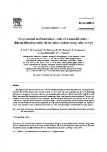
because (1) the weights occurring at each node of the partition interior to S cancel out, i.e., the value of f at each node interior to S appears either 4 times in the sum (twice with a plus sign and twice with a minus sign) or else 2 times (once with a plus sign and once with a minus sign), (2) two weights, one +1 and the other 1 occur at each node of the partition interior to an edge of S, and (3) the weights +1 occur uncontested only at the upper right and lower left corners of S and the weights 1 occur uncontested only at the other two corners of S. (To visualize this, look at Figure 1. Here we have a square, quadrasected into 4 congruent subsquares, one of

6

J. M ARSHALL ASH

which is then quadrasected into 4 congruent subsquares, This produces a partition of the original square into 7 subsquares, A; B; C; D; E; F , and G. (1) There are 4 interior nodes –a; b; c, and d; a and d are of the type that are corners of 4 partition cells and hence have 4 weights attached to them, while b and c are of the type that are corners to only 2 partition cells and hence have 2 weights attached to them. (2) There are 6 nodes interior to an edge of the original square –e; f; g; h; i, and j; each of them is common to two partition cells. (3) There are 4 nodes that are the corners of the original square –k; l; m, and n.)

Figure 1 So far, Identity (7) doesn’t seem to shed much light on our one-dimensional problem of getting an analogue of Identity (4) for second di¤erences of functions of ONE variable. Here is the connection. Associate to F (x) a function f (x; y) of two variables as follows. First, identify the point x 2 R with the line having slope 1 and passing through the point (x; x). Next let f have the value F (x) at all points of this line. In other words, for every real k, f (x k; x + k) := F (x), or, equivalently, f (x; y) := F x+y . Thus we …rst think of the domain of F as 2 being the line y = x, and then create f from F by sweeping the graph of F through three-dimensional space parallel to the vector ( 1; 1; 0). Whenever we want to move

NEW , HARDER PROOF

7

from f to its associated R-domained function F , we will use the terms shadow and project. The shadow of a point (x; y) is the point x+y 2 or, equivalently, (x; y) projects onto the point x+y . The motivation for this language comes from the fact that 2 (x; y) is orthogonally projected onto the 1-dimensional subspace f(x; y) : x = yg and then the point (x; x) is identi…ed with its …rst coordinate x. The point of all this is that is S is the above-mentioned square [a; a + p] [b; b + p], then S = p a+b F a+b 2F a+b and Identity (7) is, by some sort of miracle, 2 +p 2 + 2 +F 2 exactly the required analogue of Identity (4)! We are now ready to prove Theorem 4. Recall that a; h, and > 0 are …xed. F (a h) 2F (a)+F (a+h) < whenever h < . Find > 0 so small that for every x, h2 We will also write S for F (x h) 2F (x) + F (x + h), where S is the square [x h; x + h] [x h; x + h] and jSj = h2 , which is 41 the area of S. Now decompose the square T := a h; a + h a h; a + h into subsquares fTi g that have side P P Ti j Ti j lengths < . Then for each i, jTi j < . By Identity (7), T = Ti = jTi j jTi j. Thus, X X (8) j Tj < jTi j = jTi j = jT j ;

where the last equality amounts to the geometrically evident fact that the area of a square is the sum of the areas of the subsquares partitioning it. Dividing Inequality (8) by jT j produces the conclusion of Condition (5).

The proof of Theorem 3 can be pushed further to get the familiar calculus fact that functions with everywhere 0 derivatives are constant. Similarly we will push the proof of Theorem 4 further to get to our goal of proving Schwarz’s Theorem. To do this, we will have to partition our original square into rectangles – squares alone will not su¢ ce. If p; q > 0 and R := [a; a + p] [b; b + q] is the rectangle with lower left corner (a; b) and upper right corner (a + p; b + q), de…ne R = f (a + p; b) f (a; b + q) + f (a + p; b + q). If f is associated to R (f ) := f (a; b) a one-variable function in the usual way, f (x; y) = F x+y , then R corresponds 2 to a generalized second di¤erence studied by Riemann. In fact, R = F (x h) jp qj p+q p+q F (x k) F (x + k) + F (x + h) where x = a+b 2 + 4 ; h = 4 , and k = 4 . Also extend the above mentioned notion of shadow or projection to rectangles, saying that the projection of the rectangle R is the interval [x h; x + h] or that R projects onto this interval. Notice that many distinct rectangles may have the same shadow. Riemann pointed out, his “Schwarz derivative”is actually the special k = 0 case of the associated four-point generalized derivative which may be de…ned as limh&0;0 k 1 F (x h) F (x hk)2 kF2(x+k)+F (x+h) :[Ri, pp. 246–248] There is, of course, h 3 nothing special about 13 in this de…nition. Using Peano’s Expansion (2), we see that if F 00 (x) exists, then R = F 00 (x) h2 k 2 + o h2 . But (9)

if

k h

1 h2 , then 2 3 h k2

9 ; 8

so we may divide by h2 k 2 to see that Riemann’s limit indeed de…nes a generalized 1 derivative. Note that the denominator h2 k 2 = pq 4 is again 4 of the area of the rectangle R, so it is natural to extend the domain of de…nition of j j from squares to rectangles by setting jRj := 14 the area of R.

8

J. M ARSHALL ASH

The restriction that

k h

be bounded by

1 3

is equivalent n to othe requirement that the eccentricity e of the associated rectangle (:= max pq ; pq , i.e., the maximum ratio of its two dimensions) be bounded by 2. (Supposing that p > q so that e = pq , we …nd that hk = ee+11 , which function increases from 0 to 13 as e increases from 1 to 2.) We will call di¤erences associated with such rectangles regular. Before launching our proof of Schwarz’s Theorem, we will get one last estimate out of the way. Lemma 6. Suppose that

Then

F (x

Proof. Write

F (x

h)

F (x

k)

h)

k h

F (x

1 3

and that there is a constant C such that

2F (x) + F (x + h) 2 < C; and h2 5 2 2F (x) + F (x + k) < C: k2 5 k) h2

1 F (x + k) + F (x + h) < C: k2 2

F (x h) F (x k) F (x+k)+F (x+h) h2 k2

=

2F (x) + F (x + h) h2 + h2 h2 k 2 k2 F (x k) 2F (x) + F (x + k) : 2 2 k h k2 Take absolute values, apply the triangle inequality, bound the 2 Schwarz ratios (henceforth we will attach the adjective Schwarz to di¤erences and ratios associated with squares) by 25 C, use Implication (9) above to estimate the …rst term in curly brackets by 98 and estimate the other curly bracketed term by 19 = 89 . We get F (x

h)

F (x h) F (x k) F (x+k)+F (x+h) h2 k2

< 25 C

9 8

+

1 8

.

Second Proof of Theorem 1. As in the proof of Theorem 4, we …x a; h, and > 0 and then verify Condition (5) by …nding a partition of the square T := a h; a + h a h;na + h . o

(x+h) 2 Let 1 (x) := sup : F (x h) 2Fh(x)+F 2 5 for all h 2 (0; ) . Notice that our hypothesis forces 1 to be a positive function ( 1 (x) > 0 for every x). The reason for the bars on the h and the is to emphasize that they are to be thought of as constant for the duration of this proof. If 1 were uniformly bounded away from 0, we could simply repeat the proof of Theorem 4 and be done immediately – the problem is that 1 may be exceedingly small in a very nonuniform manner. To keep to essentials, we don’t want to waste any energy thinking about points where 1 is large, so de…ne (x) := min f 1 (x) ; 1g. Then (x) is also positive. The idea behind is that it assigns to any point x an interval (x (x) ; x + (x)) where good things happen. To make this explicit, say that a rectangle whose 4 corners project onto (x h; x h) ; (x k; x k) ; (x + k; x + k), and (x + h; x + h) is 1 …ne if R is regular (so that hk 3 ) and so small that jhj < (x). We have from Lemma 6 that j Rj 1 (10) when R is -…ne, < : jRj 2

NEW , HARDER PROOF

9

The function (x) is upper semi-continuous. In other words, for every , fx : (x) > g is closed. Since the function 1 being upper semi-continuous, and fF g [ fG g = fmin fF; Gg g show that min fF; Gg is upper semi-continuous whenever F and G are, it is enough to see why fx : 1 (x) g is closed when 0< 1. We need to show that if xn ! x and all 1 (xn ) , then 1 (x) . But F (x h) 2F (x)+F (x+h) 2 if 1 (x) < , then there is an h < such that > 5 . But F h2 is continuous at x h; x, and x + h, so we also have F (xn h) 2Fh(x2 n )+F (xn +h) > 25 for all su¢ ciently large n, contrary to 1 (xn ) . To …nish the proof of Theorem 1 it is enough to prove the following Lemma. 0 Lemma 7. Let a; h; ; T , and be as above. We can …nd a partition P P [P of T; 0 where the rectangles of P are -…ne and the rectangles of P satisfy S2P 0 j S j < 1 2 2 h . P j Rj That the Lemma su¢ ces is immediate since there holds j T j R2P jRj jRj+ P P 1 1 2 j j < 1 R2P jRj + 2 h , and the 4 area interpretation of jRj yields PS2P 0 S 2 2 R2P jRj < h . Let P be the set of x such that is bounded away from 0 on some neighborhood of x. It is immediate from the de…nition of P that P is open. Next we will show that P is dense. Let I be an open interval. Upper semi-continuity of (x) means that for each n, En := fx 2 I : (x) 1=ng is closed in I. Since I = [1 n=1 En , the Baire Category Theorem says that some Em has a non-empty interior. Any interior point of Em is in P . Say that a set N R has property ( ) if for any > 0 and rectangle R with shadow contained in N , there is a partition P of R into P -…ne rectangles and residual rectangles fKg, where the residual rectangles satisfy K2P;K residual j Kj . De…ne D by x 2 D if some neighborhood of x has property ( ). Observe that P D: (If (x) > > 0 on some interval containing the shadow of R, then let P be any partition of R into rectangles whose eccentricity is 2 and which are small enough P so that their shadows have length less than 2 . Then P partitions R so that K2P;K residual j K j = 0.) Observe also that any component of D has property ( ): Let R be any rectangle whose shadow is completely contained in D and let > 0 be given. Each point (x; y) 2 R is the center of a rectangle K whose shadow is in a neighborhood of x+y having property ( ). By compactness, R is 2 covered by …nitely many such K. Find all the lines containing some side of some such K. These lines, when intersected with R, induce a partition of R into, say, n rectangles, each of which projects into some set with property ( ). Then ( ) can be applied to each of these using n . Let C = a h; a + h nD. If C = ?, noting that all of T projects into a h; a + h D and putting = 12 h2 proves Lemma 7 and consequently Theorem 1. Suppose C 6= ?. By the Baire Category Theorem, jC is bounded away from 0 on some non-degenerate interval which intersects C. Thus we may pick an interval J so that J \ C 6= ? and is greater than the length of J on J \ C. Let I be any subinterval of J. Let B be any rectangle whose shadow is I. Let > 0. We now use Theorem 8 (which is proved in the last section of this paper) to partition B into fC1 ; :::; Cn g [ fD1 ; :::; Dm g where each rectangle Ci is regular and has its center projecting into C, and each Di has the shadow of its interior contained in D. (To apply Theorem 8, take the closed set of lines called C in

10

J. M ARSHALL ASH

Theorem 8 to be the set of all points in R2 whose shadows lie in the set called C here; similarly take D in Theorem 8 to be the set of all points projecting into the set called D here.) We further partition each Di = [a; b] [c; d] into two squares Si1 = [a; a + ] [c; c + ], and Si2 = [b ; b] [d ; d] where is chosen so small that j Si1 j + j Si2 j < =2m; and three rectangles Ti1 ; Ti2 ; Ti3 which project entirely into D. Now let P1 := fCi g ; P2 := fSij g ; P3 := fTij g. Then B is partitioned by P1 [ P2 [ P3 and since each P interval in P3 has shadow lying in D, P there is a re…nement P30 of P3 such that K2P 0 ;K residual j K j < =2. Also K2P1 ;K residual 3 P j K j = 0 since each such rectangle is -…ne, and K2P2 ;K residual j K j < =2 by P the choice of the ’s. Then P = P1 [ P2 [ P30 partitions I and K2P;K residual j K j < . Since B was an arbitrary rectangle with shadow equal to I, and since I was an arbitrary subinterval of J; J D, which is a contradiction. 3. The Partition Recall that the eccentricity of a rectangle is the longest side’s length divided by the shortest side’s length. Theorem 8. Let C be a closed set of lines with slope 1 in R2 and let D be the complement of C. Then any rectangle R can be partitioned into subrectangles such that each rectangle in the partition is of one of the following types: (c) the rectangle has eccentricity 2 and its center belongs to C: (d) the interior of the rectangle is contained in D: We will prove Theorem 8 in three stages. Lemma 9. Let C be a closed set of lines with slope 1 in R2 and let D be the complement of C. Then for any closed horizontal line segment L R2 , we can …nd a rectangle R of eccentricity 2 so that the bottom edge of R is L and so that R can be partitioned into subrectangles such that each rectangle in the partition is of one of the following types: (c) the rectangle has eccentricity 2 and its center belongs to C: (d) the interior of the rectangle is contained in D: Proof. We may assume without loss of generality that L is the line segment f(x; 0) : 0 x 1g. We must …nd a partitionable rectangle of the form [0; 1] [0; c] for some c 2 21 ; 2 . Let CY be the intersection of C with the y-axis. If some line ` in C intersects the y-axis in [3=4; 3=2], then ` also intersects the vertical line x = 1=2 at some point (1=2; p) where 1=4 p 1. Then if we let c = 2p, the rectangle R has center (1=2; p) and is of type (c) so we are done. Therefore assume that CY \ [3=4; 3=2] = ?. From now on let c = 1=2, so that R = [0; 1] [0; 1=2]. If CY \ [0; 3=4] is also empty then R is of type (d) and we are done. Therefore, let ` be the line in C with largest y-intercept 3=4. If CY \[1=2; 3=4] 6= ? then ` intersects the horizontal line y = 1=4 at some point (p; 1=4) where 1=4 p 1=2. Then R can be partitioned into two rectangles [0; 2p] [0; 1=2] and [2p; 1] [0; 1=2], where the …rst is of type (c) with center (p; 1=4) and the second is of type (d) by the maximality of `. Therefore we may assume ` intersects the y-axis at a point (0; q) where q < 1=2. The square S = [0; q] [0; q] is of type (c), and the choice of ` assures that RnS D can be partitioned into two rectangles of type (d). The square and two rectangles partition R as required.

NEW , HARDER PROOF

11

Lemma 10. Let C and D be as in the previous lemma, and let S be a square whose left edge is a vertical closed line segment L. Then there is a rectangle R S 1 such that L is also the left edge of R, the width of R is at least 12 the length of L, and R can be partitioned into rectangles, each of type (c) or (d). Proof. Assume without loss of generality that S = [0; 1] [0; 1]. We must 1 …nd a partitionable rectangle R of the form [0; d] [0; 1] for some d 2 12 ; 1 . As before, we let CY be the set of y-intercepts of lines in C. If there is a line ` with y-intercept in [3=4; 1] then ` intersects the horizontal line y = 1=2 at some point (p; 1=2) where 1=4 p 1=2. But then if we let d = 2p, R is of type (c) with center (p; 1=2) and we are done. Therefore assume that CY \ [3=4; 1] = ?. From now on, let d = 1=12 so that R = [0; 1=12] [0; 1]. By Lemma 9, we may partition in the desired way a rectangle R1 = [0; 1=12] [0; c1 ] where 1=24 c1 1=6. Applying Lemma 9 again, we partition R2 = [0; 1=12] [c1 ; c2 ] where 1=24 c2 c1 1=6. Repeated applications of Lemma 9 yield on top of each Ri = [0; 1=12] [ci 1 ; ci ] a partition of Ri+1 = [0; 1=12] [ci ; ci+1 ] where 1=24 ci+1 ci 1=6. Let n be such that cn 2 [9=12; 11=12]. This will occur for some n since ci ci 1 is always 2=12. We have therefore partitioned in the desired way a rectangle R1 [ R2 [ [ Rn = [0; 1=12] [0; cn ]. We will be done if we can partition R0 = [0; 1=12] [cn ; 1]. If int (R0 ) D then [0; 1=12] [cn ; 1] is of type (d) and we are done. Otherwise, since CY is disjoint from [3=4; 1], there is a line in C which intersects the horizontal line y = 1 in a point (p; 1) where 0 p 1=12. Since C is closed, we may let ` be the line in C with smallest such p. Since CY \ [3=4; 1] = ?, p > 0. Then the square S = [p; 1=12] [11=12 + p; 1] has center on ` and is of type (c). Again taking into account CY \ [3=4; 1] = ?, we see that the minimality of ` leads to int (R0 n S) D. Thus R0 nS can be partitioned into two rectangles of type (d). These two rectangles together with S form the desired partition of R0 and we are done. Remark 11. By using symmetry or by repeating the proof of Lemma 9 one can prove an “upside down” and 2 “sideways” versions of Lemma 9. The upside down version starts with a horizontal line segment and creates a partitionable rectangle of eccentricity 2 whose top edge is that segment. The second (respectively, third) version starts with a vertical line segment and creates a partitionable rectangle of eccentricity 2 whose right (respectively, left) edge is that segment. One can then prove 3 other versions of Lemma 10 wherein at least the right (respectively, top, bottom) 1=12 of a given square may be partitioned. The point of this remark is to justify the various appeals to symmetry which will occur in the proof of Theorem 8. Proof of Theorem 8. If C is all of R, we are done since every regular subrectangle of R is then of type (c). If D 6= ?, quadrasect R by a vertical line and a horizontal line so that the common corner of the four resulting subrectangles is in D. It will su¢ ce to show that one of these four can be partitioned as required, the arguments for the others being symmetric. Let T be the subrectangle with lower right corner d 2 D. Let S1 be the largest square contained in T containing the corner that is opposite d. If S1 contains the left edge of T , we partition a subrectangle T1 S1 using Lemma 10, that contains at least the left 1=12 of S1 . If S1 contains the top edge of T , we can similarly partition a subrectangle T1 containing at least the top 1=12 of S1 . After T1 is chosen, we let S2 be the largest square contained in the rectangle cl (T n T1 ) that contains the corner of cl (T n T1 ) opposite d, and

12

J. M ARSHALL ASH

partition a subrectangle T2 that includes at least the left 1=12 or the top 1=12 of S2 . Continuing in this manner, we get a sequence of partitioned rectangles so that, for some n, T 0 = cl (T n (T1 [ [ Tn )) is a rectangle containing d that is completely in D, so T 0 is of type (d). Thus fT1 ; T2 ; : : : ; Tn ; T 0 g is the required partition of T. References [As1] J. M. Ash, Uniqueness of representation by trigonometric series, Amer. Math. Monthly 96(1989), 873–885. [As2] ________, Multiple trigonometric series, Studies in Harmonic Analysis (J. M. Ash, ed.), of Math. Assoc. of America Studies in Mathematics, 13 (1976), pp. 76-96. [ACFR] J. M. Ash, J. Cohen, C. Freiling, and D. Rinne, Generalizations of the wave equation, Trans. Amer. Math. Soc. 338 (1993), 57–75. [AFR] J. M. Ash, C. Freiling, and D. Rinne, Uniqueness of rectangularly convergent trigonometric series, Annals of Math. 137 (1993), 145–166. [AGV] J. M. Ash, A. E. Gatto, and S Vági, A multidimensional Taylor’s theorem with minimal hypothesis, Colloq. Math. 60/61(1990), 245–252. [AW1] J. M. Ash and G. V. Welland, Convergence, summability, and uniqueness of multiple trigonometric series, Bull. Amer. Math. Soc. 77 (1971), 123–127. [AW2] ________, Convergence, uniqueness, and summability of multiple trigonometric series, Trans. Amer. Math. Soc. 163 (1972), 401–436. [Ca] G. Cantor, Beweis, das eine für jeden reellen Wert von x durch eine trigonometrische Reihe gegebene Funktion f (x) sich nur auf eine einzige Weise in dieser Form darstellen lässt, Crelles J. für Math., 72(1870), 139–142. [Ri] B. Riemann, Über die Darstellbarkeit einer Function durch eine trigonometrische Reihe, Gesammelte Abhandlungen, 2. Au‡., Georg Olms, Hildesheim, 1962, pp. 227–271. [Zy] A. Zygmund, Trigonometric Series, 2nd rev. ed., vol. 1, Cambridge Univ. Press, New York, 1959. DePaul University, Chicago, IL E-mail address : [email protected]