Hindawi Publishing Corporation Mathematical Problems in Engineering Volume 2014, Article ID 367802, 8 pages http://dx.doi.org/10.1155/2014/367802
Research Article A New Iterative Method for Linear Systems from XFEM Jianping Zhao,1,2 Yanren Hou,2 Haibiao Zheng,2 and Bo Tang3 1
College of Mathematics and System Sciences, Xinjiang University, Urumqi 830046, China School of Mathematics and Statistics, Center for Computational Geosciences, Xi’an Jiaotong University, Xi’an 710049, China 3 School of Mathematics and Computer, Hubei University of Arts and Science, Xiangyang, Hubei 441053, China 2
Correspondence should be addressed to Haibiao Zheng;
[email protected] Received 12 September 2013; Accepted 16 December 2013; Published 14 January 2014 Academic Editor: Trung Nguyen Thoi Copyright © 2014 Jianping Zhao et al. This is an open access article distributed under the Creative Commons Attribution License, which permits unrestricted use, distribution, and reproduction in any medium, provided the original work is properly cited. The extend finite element method (XFEM) is popular in structural mechanics when dealing with the problem of the cracked domains. XFEM ends up with a linear system. However, XFEM usually leads to nonsymmetric and ill-conditioned stiff matrix. In this paper, we take the linear elastostatics governing equations as the model problem. We propose a new iterative method to solve the linear equations. Here we separate two variables 𝑈 and Enr, so that we change the problems into solving the smaller scale equations iteratively. The new program can be easily applied. Finally, numerical examples show that the proposed method is more efficient than common methods; we compare the 𝐿 2 -error and the CPU time in whole process. Furthermore, the new XFEM can be applied and optimized in many other problems.
1. Introduction Many physical phenomena can be modeled by partial differential equations with singularities and interfaces. Much attention has been focused on the development of interface problem in fluid dynamics and material science. The standard finite difference and finite element methods may not be successful in giving satisfactory numerical results for such problems. Hence, many new methods have been developed. Some of them are developed with the modifications in the standard methods, so that they can deal with the discontinuities and the singularities. Peskin developed immersed boundary method (IBM) [1] basically to model blood flow in the heart. Immersed interface method (IIM) [2–6] was basically developed because of the need for a second-order accurate finite difference method to solve linear elliptic, parabolic partial differential equations in which an integral equation may not be available. IIM will give a nonsymmetric system of equations. The extended finite element method (XFEM) [7, 8] enables the accurate approximation of solutions that involve jumps, kinks, singularities, and other locally nonsmooth features within elements. This is achieved by enriching the polynomial approximation space of the classical finite
element method. The generalized finite element method (GEFM)/XFEM [9–11] has shown its potential in a variety of applications that involve nonsmooth solutions near interfaces. Among them are the simulation of cracks, shear bands, dislocations, solidification, and multifield problems. A large number of examples can be found in the real world where field quantities change rapidly over length scales that are small with respect to the observed domain. For the modeling of such phenomena, the resulting solutions typically involve discontinuities, singularities, high gradients, or other nonsmooth properties. For the approximation of nonsmooth solutions, one of the approaches is to enrich a polynomial approximation space such that the nonsmooth solutions can be modeled independently of the mesh. Methods that extend polynomial approximation spaces are called “enriched methods” in this work. The enrichment can be achieved by adding special shape functions (which are customized so as to capture jumps, singularities, etc.) to the polynomial approximation space. The total stiffness matrix consists of four parts: the FEM part, the enrich nodes part, and another two parts are the connecting parts between the real nodes and enrich nodes. Compared with FEM, the matrix size increases 𝑂(𝑁), while the FEM stiff matrix size is 𝑂(𝑁2 )(𝑁 ∼ 𝑂(ℎ−1 )).
2
Mathematical Problems in Engineering
But engineering calculations in XFEM always encountered the problem of solving ill-conditioned matrix. It made the XFEM widely. In this paper, according to the characteristics of the stiffness matrix, we use an iterative method to avoid dealing with complicated stiff matrix. First we can use the result of linear equation from standard FEM. The result can be used to be the initial value for iteration. Then we decompose the unknown values to two parts; each part is governed by two linear equations, whose dimension is smaller than the whole stiff matrix. The new programm can be easily applied. Finally, numerical examples show that the proposed method is more efficient than common methods. Furthermore, the new method works well for some problems while the common method (such as LU) fails. The new iterative method can be applied to many other problems. The outline of this paper is as follows. Section 2 introduces the XFEM. Subsequently, the main part of this paper is Section 3 that we describe a new efficient and feasible method. We also analyze the time complexity of the algorithm. In Section 4, we briefly mention details on numerical examples. A final conclusion is drawn in Section 5.
The total ordering of the element basis is given by 𝜀 and the total ordering of the nodes is given by N. The standard finite element basis is defined as follows: Bstd = ⋃ 𝑁𝐼 (𝑥) , 𝐼∈N
where 𝑁𝐼 (𝑥) is the finite element basis or shape function of node 𝐼; 𝑁𝐼 (𝑥) is assumed to be of compact support and piecewise continuously differentiable. Typically, Bstd spans the space of piecewise continuous polynomials of a specific order. The XFEM aims to alleviate the burden associated with mesh generation for problems with voids and interfaces.. It does not require the finite element mesh to conform to internal boundaries. The essence of the XFEM lies in subdividing a model into two distinct parts: mesh generation for the domain (excluding internal boundaries) and enrichment of the finite-element approximation by additional functions. A partitioning of a typical domain into its enriched and unenriched subdomains is shown in Figure 2(a). We defined the subdomain where the enrichment is applied as ΩEnr This region’s feature is that the enrichment is dominant. The elements covering ΩEnr are the enriched elements, so ⋃ Ω𝑒 = ΩEnr ,
2. The Extended Finite Element Method The basic mathematical foundation of the partition of unity finite element method (PUFEM) was discussed in [12, 13]. They illustrated that PUFEM can be used to employ the structure of the differential equation under consideration to construct effective and robust methods. The global solution of PUFEM has been the theoretical basis of the local partition of unity finite element method, to be called later the extended finite element method. The first effort for developing the extended finite element method can be traced back to 1999, [7] presented a minimal enmeshing finite element method for crack growth. They added discontinuous enrichment functions to the finite element approximation to account for the presence of the crack. The method allowed the crack to be arbitrarily aligned within the mesh, though it required enmeshing for severely curved cracks. The method was improved and called extend Finite Element Method (XFEM) in [8, 9, 11, 14–16]. In mathematics, relevant theoretical parts of doing are almost same in [17–19]. Of course, XFEM is still evolving currently and keeping the new extension about (such as fluidstructure interaction): mathematics stiff matrix remained prone to the sick. Consider a domain Ω in R𝑛 which is discredited by a set of elements Ω𝑒 such that ⋃ Ω𝑒 = Ω, 𝑒∈𝜀
(1)
(3)
𝑒∈𝜀Enr
(4)
where 𝜀Enr is the ordering of the subset of elements which are to be enriched. Any node 𝐼 for which the support of 𝑁𝐼 (𝑥) overlaps or is contained in ΩEnr is enriched node, and the set is defined by the ordering NEnr , NEnr ⊂ N. For an enrichment function 𝜓(𝑥), the enriched basis for the local partition of unity method is BEnr = Bstd ⊕ ⋃ 𝑁𝐼 (𝑥) 𝜓 (𝑥) . 𝐼∈NEnr
(5)
The approximation enriched with a local partition of unity the field 𝑢(𝑥) is given by the sum of a standard finite element approximation and a linear combination of the enriched basis functions 𝑢ℎ (𝑥) = ∑ 𝑁𝐼std (𝑥) 𝑢𝐼 + ∑ 𝑁𝐽Enr (𝑥) 𝜓 (𝑥) 𝑞𝐽 , 𝐼∈N
𝐽∈NEnr
(6)
where 𝑁𝐼std (𝑥) and 𝑁𝐽Enr (𝑥) are the shape functions for the standard part and the partition of unity, respectively; different order interpolates may be used for the standard and enriched shape functions. For example, we consider the linear elastostatics governing equations ∇ ⋅ 𝜎 + b = 0 in Ω, 𝜎 = C : 𝜀,
(7)
𝜀 = ∇𝑠 u,
and a set of nodes T = ⋃ 𝑥𝐼 . 𝐼∈N
(2)
where 𝜎 is cauchy stress and b is the body force per unit volume. The first function is called equilibrium equation. The second function is the equilibrium equation that describes
Mathematical Problems in Engineering
3
the relation of strain and displacement. The third equation is for Hooke’s law. The parameter 𝐶 implies two parameters 𝜇 = 𝐺 = 𝐸/(2(1+])) and shear elasticity, 𝜆 = 𝐸]/(1+])(1−2]) (Lam´e constants are 𝜆, 𝜇 and Poisson’s ratio is ]). Consider u=u
on Γ𝑢 , on Γ𝑡 ,
𝜎⋅n=t 𝜎 ⋅ n𝑖ℎ = 0 [𝜎 ⋅
n𝑖𝐼 ]
on Γℎ𝑖 (𝑖 = 1, 2, . . . , 𝑚) ,
=0
on
Γ𝐼𝑖
(8)
1 𝜓Ramp = { 1 − 2𝜑
(𝑖 = 1, 2, . . . , 𝑛) .
The boundary Γ is composed of the sets Γ𝑢 , Γ𝑡 , Γℎ𝑖 , and Γ𝐼𝑖 such that Γ = Γ𝑢 ∪ Γ𝑡 ∪ Γℎ𝑖 ∪ Γ𝐼𝑖 ,
(9)
where 𝑛 is the unit outward normal to Ω and 𝑢 and t are prescribed displacements and traction, respectively. The weak formulation of (12) is well known and reads as follows: find 𝑢 ∈ 𝑉 such that ∫ 𝜎 (u) : 𝜀 (k) 𝑑Ω = ∫ b ⋅ k𝑑Ω + ∫ t ⋅ k𝑑Γ ∀V ∈ 𝑉0 . Ω
Ω
Γ𝑡
(10) Here 𝑉 = 𝐻1 (Ω) and 𝑉0 = {V ∈ 𝑉 : V = 0 on Γ𝑢 }. For the finite element discretization, let 𝜏ℎ be a regular rectangular element of domain Ω and define the mesh parameter ℎ = max𝑇∈𝜏ℎ {diam(𝑇)}. Consider the Bubnov-Galerkin implementation for the XFEM in two-dimensional linear elasticity. In the XFEM, finite-dimensional subspaces 𝑉ℎ ⊂ 𝑉 and 𝑉0ℎ ⊂ 𝑉0 are used as the approximating trial and test spaces. The finite dimensional space 𝑉ℎ is given by 𝑉ℎ = { V ∈ 𝑉 : V|𝑇 ∈ 𝑄𝑘 (𝑇) , ∀𝑇 ∈ 𝜏ℎ } .
(11)
The weak form of the discrete problem can be stated as follows: find 𝑢ℎ ∈ 𝑉ℎ such that ∫ 𝜎 (uℎ ) : 𝜀 (kℎ ) 𝑑Ω = ∫ b ⋅ kℎ 𝑑Ω + ∫ t ⋅ kℎ 𝑑Γ ∀Vℎ ∈ 𝑉0ℎ ⊂ 𝑉0 ,
(12)
where 𝑉ℎ ⊂ 𝑉 and 𝑉0ℎ ⊂ 𝑉0 . In a Bubnov-Galkerkin procedure, the trial function 𝑢ℎ and the test function Vℎ are represented as linear combinations of the same shape functions. The trial and test functions are uℎ (x) = ∑𝜙𝐼 (x) u𝐼 + ∑𝜙𝐽 𝜓 (𝜑 (x)) a𝐽 , 𝐽
(13)
kℎ (x) = ∑𝜙𝐼 (x) k𝐼 + ∑𝜙𝐽 𝜓 (𝜑 (x)) b𝐽 , 𝐼
(14)
𝜓Step = {
1 𝜑 > 0, −1 𝜑 ≤ 0.
(15)
This enrichment function can yield a continuous or discontinuous solution across the interface but requires Lagrange multipliers to apply the Dirichlet jump condition. On substituting the trial and test functions form (17), and using the arbitrariness of nodal variations, the following discrete system of linear equations is obtained: Kd = F,
(16)
K𝐼𝐽 = ∫ B𝑇𝐼 CB𝐽 𝑑Ω,
(17)
F𝐼 = ∫ 𝜙̂𝐼 t 𝑑Γ + ∫ 𝜙̂𝐼 b 𝑑Ω.
(18)
where Ωℎ
Γ𝑡ℎ
Ωℎ
𝜙̂𝐼 ≡ 𝜙𝐼 for a finite-element displacement degree of freedom, and 𝜙̂𝐼 ≡ 𝜙𝐼 𝜓 for an enriched degree of freedom. In the above equations, C is the constitutive matrix for an isotropic linear elastic material: 𝜆 + 2𝐺 1 0 1 𝜆 + 2𝐺 0 ) , 0 0 𝐺
(19)
and the matrix B𝐼 is given by
Γ𝑡ℎ
𝐼
𝜑>0 𝜑 ≤ 0.
This enrichment function yields only continuous solutions. The advantage is that it automatically satisfies the continuity condition [𝑢] = 0 and does not require the use of Lagrange multipliers. The step-enrichment function is defined as
𝐶=(
Ωℎ
Ωℎ
interface. 𝜙𝐼 (x) are the finite-element shape functions, 𝜑(x) is the level set function, and 𝜓(𝜑(x)) is the enrichment function for material interface. There are several kinds of enrichment functions, such as abs-enrichment function, step-enrichment function, and Ramp-enrichment function. The choice of function is based on the behavior of the solution near the interface. The Ramp function is defined as
𝐽
where 𝐼 denotes the set of all nodes in the mesh and 𝐽 = {𝑗 ∈ 𝐼 : 𝑂𝜀 x𝑗 ∪ Γ ≠ 0}(𝜀 ≤ ℎ) denotes the set of nodes near the
𝜙̂𝐼,𝑥 B𝐼 = ( 0 𝜙̂𝐼,𝑦
0 𝜙̂𝐼,𝑦 ) . 𝜙̂𝐼,𝑥
(20)
We can get the integral terms, and the matrices computed from the integral terms are block matrices of the form 𝐾𝑈𝑈 𝐾𝑈𝐴 𝐾 = ( 𝐴𝑈 𝐴𝐴) , 𝐾 𝐾
𝐹𝑈 𝐹 = ( 𝐴) , 𝐹
𝑈 𝑑 = ( ). Enr The next step is solving the linear equations system.
(21)
4
Mathematical Problems in Engineering
3. The Program for Solving the Equation
(3) The original matrix deposit triangular matrix and diagonal matrix deposit area can overlap, thus avoiding to take up a lot of the middle unit of work, saving memory.
We need to solve the following equations: 11 12 1 𝑀𝑛×𝑛 𝑈𝑛×1 𝑅𝑛×1 𝑀𝑛×𝑚 ( 21 ) ( ) = ( 22 2 ). Enr𝑚×1 𝑀𝑚×𝑛 𝑀𝑚×𝑚 𝑅𝑚×1
(22)
Here 𝑛 ∼ 𝑂(𝑁2 ) and 𝑚 ∼ 𝑂(𝑁), the block matrix 𝑀11 is same in FEM and (𝑀21 ) = 𝑀12 are sparse matrix. We must point out that the matrix 𝑀12 has up to 𝑚2 nonzero elements. We can use the modified program, in (22) can be converted to two sub-problems: to solve (𝑀22 )−1 and solve 𝑈 by 𝑛-order linear equations. Now, we list the detailed steps. Algorithm 1. (i) We use the ordinary method to solve 𝑀11 𝑈(0) = 𝑅1 ,
(23)
the results for the FEM equation and set the result as 𝑈(0) , 𝐸(0) = 0. The matrix 𝑀11 is block tridiagonal symmetric, sparse matrix. There are a lot of methods to solve this equation efficiently. (ii) Solve the small scale equation 𝑀22 Enr(𝑖+1) = 𝑅2 − 𝑀21 𝑈(𝑖) ,
𝑖 = 0, 1, . . . .
(24)
22
The matrix 𝑀 is a sparse tridiagonal, where the dimension is much smaller than 𝑀11 . This equation can be solved quicker than (i). (iii) Then we use (25) to solve 𝑈(𝑖+1) ; 𝑀11 𝑈(𝑖+1) = 𝑅1 − 𝑀12 Enr(𝑖+1) ,
𝑖 = 0, 1, . . . .,
(4) This solution can be extended to block direct solution. (5) With the iterative method, it is easy to build and test the general program and you can more accurately estimate the computation time; the user is relatively easy to grasp the algorithm process. Also if we using in [21] to solve the equation, ((2𝑁)2 + 4𝑁) equations use LU solver which need 𝑂((2𝑁)2 + 4𝑁)3 Multiplication, here if the number of iterations is 𝐼, we use up to 𝑂((2𝑁)6 + (4𝑁)3 ) multiplications.
4. Numerical Test In this section, we report two experiments to verify the efficacy and accuracy of the new iterative method in XFEM. We use Matlab and modify software [22] to demonstrate Algorithm 1. For the convenience of presentation, we introduce the following notations: SFEM means the standard finite element method; XFEM means the extended finite element method; ℎ means the mesh size; GMRES means the generalized minimal residual iterative method; 𝐿 2 -error means ‖𝑢ℎ − 𝑢‖0 ;
(25)
𝐸ℎ means the 𝐿 2 -error when the mesh size equals ℎ;
the computation time complexity is the same with the first one. (iv) If the norm ‖𝑈(𝑖+1) − 𝑈(𝑖) ‖ ≤ 𝑤 or 𝑖 > 𝐼max (giving the maximum iterative times), output the result 𝑈 = 𝑈(𝑖+1) , Enr = Enr(𝑖+1) . Else, return to step (ii). In this part, we can use the common FEM solver such as LU or other useful solvers. We do not change the stiffness matrix 𝑀11 and 𝑀22 , these two matrixes are symmetric, positive, definite and banded. We can compute easily for (23), (24), (25). The matrix conditions is not changed; K(𝑀11 ) = 𝑂(ℎ−2 ) [17]. First of all, the store can choose a one-dimensional. We can choose a one dimensional storage when we use triangular decomposition for the matrix 𝑀.
iterations mean the iterative times in the algorithm;
Remark 2. If the matrix 𝑀11 and 𝐴22 are not tridiagonal, we often use LU or GMRES method [20] to solve (23), (24), and (25). The iteration has the following advantages. (1) Other than the half bandwidth of zero elements do not have storage, nor involved in the calculation, the amount of storage crunch, the impact of rounding error is relatively small, even if it is ill-conditioned matrix, we often obtain a higher accuracy. (2) The operator only uses FEM linear equation solver; it is a simple calculation.
orders mean the numerical error order by XFEM: orders =
log (𝐸ℎ1 /𝐸ℎ2 ) log (ℎ1 /ℎ2 )
.
(26)
Here ℎ1 ≤ ℎ2 . First, we list Example 1 for one-dimensional problems. Example 1. The exact solution is 1 (𝑥 − 0.5)2 (𝑥 − 0.5) (𝑘1 − 𝑘2 ) { { − + , − { { 2𝑘 4𝑘 (𝑘 + 𝑘 ) 4 (𝑘 { 2 2 2 1 2 + 𝑘1 ) { { { { { if 𝑥 ∈ Ω1 , 𝑢={ 2 (𝑥 − 0.5) (𝑘1 − 𝑘2 ) 1 { (𝑥 − 0.5) { { − − + , { { 2𝑘 4𝑘 (𝑘 + 𝑘 ) 4 (𝑘 { 1 1 2 1 2 + 𝑘1 ) { { { if 𝑥 ∈ Ω2 . {
(27)
Here Ω1 = [0, 0.5] and Ω2 = (0.5, 1] the coefficient 𝑘 = 1, if 𝑥 ∈ Ω1 , 𝑘 = 10, if 𝑥 ∈ Ω2 . And 𝐹 is point force from the righ; 𝐹 = 10. We use Figure 1 to describe the 𝐿 2 error change when we use different ℎ. We can easily see that, when the step is smaller than 1/80, the whole computing time has economized one order of magnitude in Example 1.
Mathematical Problems in Engineering
5 10−3
10−2
10−4
10−3
ErrorL2
Time
10−5
10−4
10−6 10−7 10−8 10−9
102
103
104
10−10 101
102
104
103 1/h
1/h
ErrL2 for LU ErrL1 for iterative method
ErrL2 for LU ErrL2 for iteration (a)
(b)
Figure 1: (a) The comparison of time by iteration and LU with different mesh. (b) The comparison of 𝐿 2 -error by iteration and LU with different mesh. 0
1
100
0.8
200
0.6
y
0.4
300
0.2
400
0
500
−0.2
600
−0.4
700
−0.6
800
−0.8
900
−1
1000 −1 −0.8 −0.6 −0.4 −0.2
0 x
0.2
0.4
0.6
0.8
1
0
200
400
600
800
1000
nz = 17803
(a)
(b)
Figure 2: (a) All nodes and enrichment nodes (in red color); 𝑁 = 20; (b) distribution map of nonzero elements in whole matrix 𝑀; 𝑁 = 20.
Example 2. For the two-dimensional solid test, we use the same enrichment function and shape function to compute (4). We define Ω = [0, 1] × [0, 1] with the material interface Γ : 𝑥2 + 𝑦2 = 𝑎2 = 0.1608.
(28)
Let Young’s modulus and Poisson’s ratio in Ω1 = {(𝑥, 𝑦) ∈ Ω | 𝑥2 + 𝑦2 ≤ 0.4042 }
(29)
be 𝐸1 = 100, ]1 = 0 and let those in 1 Ω2 = {(𝑥, 𝑦) ∈ Ω | 𝑥2 + 𝑦2 ≤ } 4
(30)
be 𝐸2 = 10, ]2 = 0, but area force in domain 𝑓𝑥 = 𝑓𝑦 = 0.
6
Mathematical Problems in Engineering Table 1: DOF, sparsity of matrix, and condition number of linear equation by FEM and XFEM for Example 2.
ℎ 1 20 1 40 1 60 1 80 1 100
DOFFEM
DOFXFEM
condsFEM
condsXFEM 4
Sparsity of matrix (%) 4
882
1018
1.7627 × 10
7.90617 × 10
1.72
3362
3626
3.75035 × 10⁴
3.20917 × 10⁵
0.4774
12800
13120
1.02381 × 10⁵
1.30023 × 10⁶
0.222
12800
13120
1.02381 × 10⁵
1.30023 × 10⁶
0.13
25600
26240
4.07606 × 10⁵
5.23974 × 10⁶
0.0829
Table 2: The CPU time for different solvers in Example 2. ℎ 1 20 1 40 1 60 1 80 1 100
FEMLU
XFEMiteration
XFEMLU (s)
XFEMGMRES (s)
1.2166
1.3129
2.6019
2.1449
5.7133
6.5198
7.3678
8.9494
17.8348
20.6117
27.2810
26.6332
54.3007
59.0695
70.4340
70.7011
137.89
145.92
165.1256
166.5808
Table 3: The comparison of 𝐿 2 -error with different solvers for Example 2. ℎ 1 20 1 40 1 60 1 80 1 100
FEMLU
XFEMLU (s) −2
−3
6.4292 × 10
6.3756 × 10
6.3756 × 10⁻³
2.1032 × 10⁻²
1.7108 × 10⁻³
1.7097 × 10⁻³
1.7092 × 10⁻³
1.4089 × 10⁻²
7.7599 × 10⁻⁴
7.7595 × 10⁻⁴
7.7554 × 10⁻⁴
1.0317 × 10⁻²
4.1781 × 10⁻⁴
4.1434 × 10⁻⁴
4.1733 × 10⁻⁴
8.2802 × 10⁻³
2.7344 × 10⁻⁴
2.7002 × 10⁻⁴
2.7295 × 10⁻⁴
𝑎 𝑟 𝑎 ( (𝜅 + 1) cos 𝜃 + 2 ((1 + 𝜅) cos 𝜃 + cos 3𝜃) 8𝜇 𝑎 𝑟 −2
𝑎3 cos 3𝜃) , 𝑟3
𝑎 𝑟 𝑎 V= ( (𝜅 − 3) sin 𝜃 + 2 ((1 − 𝜅) sin 𝜃 + sin 3𝜃) 8𝜇 𝑎 𝑟 −2
𝑎3 sin 3𝜃) . 𝑟3
(31)
−3
XFEMiteration (s)
4.2101 × 10
We denote 𝑟 = √𝑥2 + 𝑦2 and tan 𝜃 = 𝑦/𝑥, and the exact solution is 𝑢=
XFEMGMRES
Plate with a circular hole. Figure 2(b) shows the consistent rectangular subdivision and labels the nodes which need to be extended. The CPU time we counted is the total time for the entire programm running. Table 1 shows the linear equation scale and the condition numbers of FEM and XFEM, the density of sparse matrix show the matrix is sparse. It can be easily find the condition number of XFEM is bigger than that of FEM. The CPU times are also compared with LU solvers and GMRES in Table 2. The cheapest is LU by FEM and the new iterative method is the second cheapest; however, the error for LU by FEM is the biggest in all methods. Table 3 shows an 𝐿 2 -error comparison between the new iterative method and other solvers. And the numerical 𝐿 2 -error is nearly 𝑂(ℎ2 ). 𝐿 2 -error, order, and iterations are given in Table 4.
Mathematical Problems in Engineering
7
Table 4: 𝐿 2 -error, order, CPU time, and iterations by XFEM with the new iterative method for Example 2. ℎ 1 20 1 40 1 60 1 80 1 100
ErrorXFEM
Orders
CPUXFEM (s)
Iterations
\
1.313
24
1.7092 × 10⁻³
1.8992
6.52
19
7.7554 × 10⁻⁴
1.9489
20.61
19
4.1733 × 10⁻⁴
2.1541
59.07
19
2.7295 × 10⁻⁴
1.9028
145.92
18
−3
6.3754 × 10
5. Conclusion In this paper, we discuss how to use XFEM for the stiff matrix ill-conditioned and came to the following conclusions. Firstly, we found why some of problems cannot be computed by XFEM; the stiff matrix is not then symmetric and illconditioned. So, a lot of storage space is wasted. The time of computing XFEM equation is longer, which cannot be computed in certain subdivision. Secondly, we use XFEM for solving two-dimensional solid test; when solving the XFEM equations, the iterative method and the standard finite element equations solver are adopted, so that we change the problems into solving the smaller scale equations and standard finite element stiffness matrix need not be changed. Finally, numerical examples show that the proposed method is more efficient than the common method. We can use this programm in many other interface problems later. Besides, we also consider combining the stable GFEM with our iterative method in the future. And it is believed that the XFEM can be widely used in more problems in fluid dynamics and material science. The calculation module in some software can be improved for users.
Conflict of Interests The authors declare that there is no conflict of interests regarding the publication of this paper.
Acknowledgments The author also thanks the anonymous reviewers for their comments in improving the paper. This research was supported by the special funds for NSFC (1127313, 11171269, 11201369, and 61163027) and the Ph.D. Programs Foundation of the Ministry of Education of China (Grant no. 20110201110027), and it was partially subsidized by the Fundamental Research Funds for the Central Universities (Grant nos. 08142003 and 08143007).
References [1] C. S. Peskin, “Flow patterns around heart valves: A numerical method,” Journal of Computational Physics, vol. 10, no. 2, pp. 252–271, 1972.
[2] R. J. LeVeque and Z. L. Li, “The immersed interface method for elliptic equations with discontinuous coefficients and singular sources,” SIAM Journal on Numerical Analysis, vol. 31, no. 4, pp. 1019–1044, 1994. [3] Z. Li, K. Ito, and M.-C. Lai, “An augmented approach for Stokes equations with a discontinuous viscosity and singular forces,” Computers & Fluids, vol. 36, no. 3, pp. 622–635, 2007. [4] A. L. Fogelson and J. P. Keener, “Immersed interface methods for Neumann and related problems in two and three dimensions,” SIAM Journal on Scientific Computing, vol. 22, no. 5, pp. 1630–1654, 2000. [5] Z. Li, “The immersed interface method using a finite element formulation,” Applied Numerical Mathematics, vol. 27, no. 3, pp. 253–267, 1998. [6] H. Huang and Z. Li, “Convergence analysis of the immersed interface method,” IMA Journal of Numerical Analysis, vol. 19, no. 4, pp. 583–608, 1999. [7] N. Mo¨es, J. Dolbow, and T. Belytschko, “A finite element method for crack growth without remeshing,” International Journal for Numerical Methods in Engineering, vol. 46, no. 1, pp. 131–150, 1999. [8] N. Sukumar, D. L. Chopp, N. Mo¨es, and T. Belytschko, “Modeling holes and inclusions by level sets in the extended finiteelement method,” Computer Methods in Applied Mechanics and Engineering, vol. 190, no. 46-47, pp. 6183–6200, 2001. [9] J. Chessa, H. Wang, and T. Belytschko, “On the construction of blending elements for local partition of unity enriched finite elements,” International Journal for Numerical Methods in Engineering, vol. 57, no. 7, pp. 1015–1038, 2003. [10] T.-P. Fries and T. Belytschko, “The extended/generalized finite element method: an overview of the method and its applications,” International Journal for Numerical Methods in Engineering, vol. 84, no. 3, pp. 253–304, 2010. [11] T. Belytschko, R. Gracie, and G. Ventura, “A review of extended/generalized finite element methods for material modeling,” Modelling and Simulation in Materials Science and Engineering, vol. 17, pp. 1–24, 2009. [12] I. Babuˇska and J. M. Melenk, “The partition of unity method,” International Journal for Numerical Methods in Engineering, vol. 40, no. 4, pp. 727–758, 1997. [13] J. M. Melenk and I. Babuˇska, “The partition of unity finite element method: basic theory and applications,” Computer Methods in Applied Mechanics and Engineering, vol. 139, no. 1–4, pp. 289–314, 1996. [14] T.-P. Fries and T. Belytschko, “The intrinsic XFEM: a method for arbitrary discontinuities without additional unknowns,”
8
[15]
[16]
[17]
[18]
[19]
[20]
[21]
[22]
Mathematical Problems in Engineering International Journal for Numerical Methods in Engineering, vol. 68, no. 13, pp. 1358–1385, 2006. J.-Y. Wu, “Unified analysis of enriched finite elements for modeling cohesive cracks,” Computer Methods in Applied Mechanics and Engineering, vol. 200, no. 45-46, pp. 3031–3050, 2011. H. Sauerland and T.-P. Fries, “The extended finite element method for two-phase and free-surface flows: a systematic study,” Journal of Computational Physics, vol. 230, no. 9, pp. 3369–3390, 2011. I. Babuˇska and U. Banerjee, “Stable generalized finite element method (SGFEM),” Computer Methods in Applied Mechanics and Engineering, vol. 201–204, pp. 91–111, 2012. T. Strouboulis, I. Babuˇska, and K. Copps, “The design and analysis of the generalized finite element method,” Computer Methods in Applied Mechanics and Engineering, vol. 181, no. 1–3, pp. 43–69, 2000. T. Strouboulis, K. Copps, and I. Babuˇska, “The generalized finite element method: an example of its implementation and illustration of its performance,” International Journal for Numerical Methods in Engineering, vol. 47, no. 8, pp. 1401–1417, 2000. Y. Saad and M. H. Schultz, “GMRES: a generalized minimal residual algorithm for solving nonsymmetric linear systems,” SIAM Journal on Scientific and Statistical Computing, vol. 7, no. 3, pp. 856–869, 1986. G. Meurant, “A review on the inverse of symmetric tridiagonal and block tridiagonal matrices,” SIAM Journal on Matrix Analysis and Applications, vol. 13, no. 3, pp. 707–728, 1992. Copyright (c), Thomas-Peter Fries, RWTH Aachen University, 2010.
Advances in
Operations Research Hindawi Publishing Corporation http://www.hindawi.com
Volume 2014
Advances in
Decision Sciences Hindawi Publishing Corporation http://www.hindawi.com
Volume 2014
Journal of
Applied Mathematics
Algebra
Hindawi Publishing Corporation http://www.hindawi.com
Hindawi Publishing Corporation http://www.hindawi.com
Volume 2014
Journal of
Probability and Statistics Volume 2014
The Scientific World Journal Hindawi Publishing Corporation http://www.hindawi.com
Hindawi Publishing Corporation http://www.hindawi.com
Volume 2014
International Journal of
Differential Equations Hindawi Publishing Corporation http://www.hindawi.com
Volume 2014
Volume 2014
Submit your manuscripts at http://www.hindawi.com International Journal of
Advances in
Combinatorics Hindawi Publishing Corporation http://www.hindawi.com
Mathematical Physics Hindawi Publishing Corporation http://www.hindawi.com
Volume 2014
Journal of
Complex Analysis Hindawi Publishing Corporation http://www.hindawi.com
Volume 2014
International Journal of Mathematics and Mathematical Sciences
Mathematical Problems in Engineering
Journal of
Mathematics Hindawi Publishing Corporation http://www.hindawi.com
Volume 2014
Hindawi Publishing Corporation http://www.hindawi.com
Volume 2014
Volume 2014
Hindawi Publishing Corporation http://www.hindawi.com
Volume 2014
Discrete Mathematics
Journal of
Volume 2014
Hindawi Publishing Corporation http://www.hindawi.com
Discrete Dynamics in Nature and Society
Journal of
Function Spaces Hindawi Publishing Corporation http://www.hindawi.com
Abstract and Applied Analysis
Volume 2014
Hindawi Publishing Corporation http://www.hindawi.com
Volume 2014
Hindawi Publishing Corporation http://www.hindawi.com
Volume 2014
International Journal of
Journal of
Stochastic Analysis
Optimization
Hindawi Publishing Corporation http://www.hindawi.com
Hindawi Publishing Corporation http://www.hindawi.com
Volume 2014
Volume 2014