A New Look at Classification of Transformer Normal and Abnormal Currents Mohamed Abdel-Hafez Department of Electrical Engineering, College of Engineering, United Arab Emirates University, P.O.Box 17555, Al-Ain, UAE, email:
[email protected] .
Ahmed .M. Gaouda Department of Electrical Engineering, College of Engineering, United Arab Emirates University, P.O.Box 17555, Al-Ain, UAE, email
[email protected] .
Abstract— The paper proposes an enhanced wavelet-based feature extraction technique to classify transformer inrush currents (TIC) and transformer internal faults (TIF). The proposed tool utilizes the number of wavelet coefficients of local maxima as current signal slides into Kaiser’s window. The general pattern of number of coefficients of local maxima at the first three resolutions are used to design a new automated tool for monitoring and classifying abnormal conditions in power transformers. The proposed monitoring technique is evaluated using large data sets.
Transformer internal fault (TIF) currents generate pure fundamental component and a possible decaying dc component [2]. Harmonic in faults are generally small and even [1]. The strength of these harmonics depends on the fault instant, fault phase-shift, transformer circuit model and connected load. The features extracted during transformer internal faults (TIF) are similar to that during transformer inrush currents (TIC) and an accurate and rapid discrimination between them is essential for transformer monitoring tools. The wavelet analysis has emerged as a powerful tool for signal processing in different power system applications [6], [7] including analysis of transformer faults and inrush currents. In [5] several features were derived from wavelet packet (WP) transform. The proposed technique utilized a signal combined from the product of a fault current and a prefault voltage. The sampling rate is selected as 20kHz and the signal is decomposed up to 3rd level that covers frequency band up to 10kHz. The proposed TIC classification features are described based on the sum of some wavelet coefficients generated utilizing WP transform. However, the sign of these coefficients depends on the signal under process and their summation may produce different results for similar signals. Furthermore, Daubechies 1 (db1) is used in the decomposition process which has two vanishing moments (two coefficients) and allows wide spread (leakage) of signal’s energy into adjacent resolutions. In [8] a technique combining wavelet transform and neural network is presented. The proposed technique concentrated on the first 3 resolution levels (12.51.562kHz) and used the detected sharp spikes localized at these resolutions in the classification process. The proposed technique utilizes the reconstructed version of the signals using Daubechies 4 (db4 with 8 coefficients). Similarly, in [3] the spikes localized at first 4 resolutions are used to monitor TIF and TIC cases. The duration of these spikes and their decaying nature are used in the classification process. The detail coefficients using Daubechies 4 are used in the analysis and classification process. The two proposed techniques in [8] and [3] monitor the spikes at high resolution levels, however, these spikes might be generated due to any fast changes such as switching phenomenon or load changes. Further, there are some cases where the variation in the TIC is smooth and hence no periodic spikes would be detected at high frequency bands. Moreover convolution technique (a tool of DWT) and data
Index Terms — Inrush current, Transformer Faults, Kaiser’s Window, Multi-resolution analysis, and Wavelet transform.
I. INTRODUCTION Monitoring and classifying transformer inrush currents (TIC) and transformer internal faults (TIF) are still challenging problems for distribution system engineers. There is always a possibility for false tripping caused by the magnetizing inrush current [1]-[3]. Although the magnitude of the magnetizing current is only 1–2% of the transformer rated current under the steady state operating conditions, the inrush current may approach short-circuit levels and cause fuses, reclosers, or relays to falsely operate [4]. These currents may persist from about 10 cycles to as long as 1 minute in very high-inductive circuits [1], [5]. The transformer inrush current (TIC) depends on many factors including the instant of connecting the source, residual flux, type of winding connections, core type, core material and load characteristics [1], [2]. This current is characterized as a non-stationary, harmonic distorted with positive or negative dc offset. The proportion of harmonics varies as the cycles of TIC passes. The 2nd harmonic component of inrush current is dominant and may reach to 15% or more of the fundamental. In recent years, improvements in core material and design are resulting in TIC with less distortion where a 2 nd harmonic component being as low as 7%. [1]. Transformer inrush current (TIC) may occur when a transformer is first energized or reenergized after a short period of interruption. It may also occur after voltage returns to normal value following a fault or a voltage dip [6] or may result from paralleling a second transformer with a transformer already in operation [1].
978-1-4244-5795-3/10/$26.00 ©2010 IEEE
830
sliding process may generate such spikes at the start and end of the data processing window. In [9] the second harmonic component is used as the characteristic component of the TIC. Wavelet based feature extraction scheme is performed by decompose the currents and concentrate on the resolution level that cover the second harmonic components. Detecting two successive peak and bottom and counting the number of samples between them is used to identify the phase subjected to TIC in three phase transformers. The proposed technique utilizes the reconstructed version of the signals using Daubechies 4. In [10] a wavelet-based decision trees, for feature extraction, and a pattern recognition technique are combined to generate TIC features for transformer protection. The detail coefficients, extracted by Haar wavelet (Daubechies 1), are used as additional features for the pattern recognition tool. In this paper, we use a recent proposed wavelet-based technique [11, 12] for accurately and efficiently discriminates between TIC and TIF cases. The monitoring process is enhanced by processing signals as data sliding into Kaiser’s window. A small set of coefficients of local-maxima that represent most of signal’s energy are used to classify different cases. Processing data through Kaiser's window increases the similarity between processed signals and the selected mother wavelets, hence different wavelets will result similar features. No reconstruction process is required in the proposed technique. Only one coefficient and its index at each resolution level are used to detect and measure non-stationary variation of TIC and TIF cases. The maximum coefficient at the 50Hz resolution is used to monitor the signal's magnitude in order to take protection action in case of faults. The paper is organized as follows. An introduction to wavelet multi-resolution analysis (WMRA) is discussed in Section II. The proposed enhancement wavelet monitoring technique is also presented in this section. Wavelet-bases feature extraction is presented in Section III. The proposed pattern classification method of TIC and TIF is discussed in Section IV. Section IV presents data generation and analysis. Conclusion and references are presented in Sections VII, VIII simultaneously. II. WAVELET MULTI-RESOLUTION ANALYSIS Applying wavelet multi-resolution analysis, one can decompose a current signal i( t ) at different resolution levels and present it as a series of approximate c j ( k ) and detail
d j ( k ) expansion coefficients. Fig. 1 shows a one stage of wavelet decomposition process. The sets of expansion coefficients at a lower resolution can be mathematically calculated as: ho ( m 2k ) c j ( m ) (1) c j1 ( k )
m
d j 1( k )
h ( m 2k ) c ( m ) 1
j
(2)
m
where ho ( k ) and h1( k ) present the coefficients of the selected scaling and wavelet functions. The current, i( t ) L2 ( R ) , can
831
be presented as a series of expansion coefficients and a combination of the scaling function ( t ) and wavelets function ( t ) as: J 1
i( t )
c ( k ) ( t k ) d ( k )2 o
j
k
k
j/2
(2 jt k )
(3)
j 0
Generating a windowing version of the signal increases the similarity between the signal under process and the selected wavelet function. Kaiser’s window of length wN is selected in the windowing process, which is mathematically presented as: w[ n ]
I o { [ 1 ( n u ) 2 / u 2 ] 0 .5 } I o ( ( 0 , ))
(4)
for n 0 ,1,....,wN 1
where I o ( x ) is the modified Bessel function, u is the midpoint of the window function and 0 10 . The advantage of selecting Kaiser’s window comes from the ability to adjust the window shape by changing [16], [17]. 0.8
Wavelet Function
0.4 0 -0.4 -0.8 0
15
30
15
30
0.8 0.4
Scaling Function
0 -0.2 0
Fig.1. Wavelet transform detail and approximate coefficients at first resolution (a ) level H(ω) H1( )
Ho ( ) Using db Mallat’s algorithm, the set of expansion coefficients 4 of a windowing version of the signal at certain resolution level / 2 can be defined as: H(ω) H1( ) wd j ( k )H (5) o ( ) h1 ( m 2 k ) wc j 1 ( m ) db40
m
H(ω)
/ 2
III. WAVELET-BASED FEATURES EXTRACTION H1( ) Ho ( ) coifextraction 5 Feature is a preprocessing operation that transforms a pattern from its original form to a new form / 2 suitable for further processing.(b Mapping the data of the ) distorted signal into a windowed-wavelet domain is the first step in performing the proposed feature extraction process. The number of coefficients of local maxima extracted at the first three resolution levels is the main features of the classification technique. The goal of this stage is to represent TIC or TIF cases in terms of a manageable set of coefficients that can classify different disturbances. As data slides into Kaiser’s window, the coefficients of local maxima and their indices localized at each resolution level are defined. The absolute value of the detail coefficients ( | wd j | ) are used to localize either positive or negative expansion coefficients that carry most of the signal’s energy. For the set of wavelet coefficients localized at certain resolution level, a local maxima takes on the largest value
among all coefficients in the immediate vicinity. Therefore, a coefficient | wd j ( k ) | is a local maxima of some neighborhood coefficients if | wd j ( k ) | > | wd j ( k 1 ) | . The coefficients of local maximum are presented as: (6)
[ wd j ( N j )]loc local maxima [ | wd j ( k )| ]
The proposed classification technique presented in this paper is evaluated using 20 sets of simulated TIC and TIF data. The event time instant, fault impedance, transformer size and saturation curve, and source and load impedances are varied to generate different simulated signals. The proposed technique is applied on the simulated data and the magnitude of signal ( Mag j ) at each resolution level and
If MAX (Nlos) > TH_Nloc then ; State = Clear Alarm; %TIC case Else State = Alarm ; % TIF case End The threshold value TH_Nloc can be roughly taken as 10 based of the 20 set of simulations presented in Fig. 2. The major disadvantage of this rule is the response time which is very long and we have to look for quicker rule to detect the faults. Fig.3 shows a model pattern for Nloc. We will define the rate of change of Nloc w.r.t wc at the ith instant is: Ri N i / i wc (7)
the numbers of coefficients of local maxima ( N loc ) are monitored. Fig. 2 shows the pattern of the number of coefficients of local maxima ( N loc ) at the first three resolution levels as w c changes with a sliding rate of 1.5 cycles. The features are extracted under different operation conditions.
Ni
60
60
N loc
N loc
[ wd 1 ,2 ,3 ] loc
50
[ wd 1 ,2 ,3 ] loc
50
TIC
TIC
40
40 30
N loc
30
[ wd 1 ,2 ,3 ] loc
20
TIF
20
0 0.2
0.4
0.6
0.8
60
N loc 50
0 0.2
wc 1
20
0.4
It is clear for Fig. 2 that Ri for TIC and TIF can be greatly separated within the first 5 samples therefore Ri was calculated for all scenarios and for the 20 sets of simulations to come up with a fast classification rule between TIC and TIF.
0.6
0.8
wc 1
[ wd 1 ,2 ,3 ] loc
70
TIC
V. DATA ANALYSIS
TIC
60
Using the 20 sets of simulated TIC and TIF and the patterns generated for Nloc at first three resolution levels we generated Ri for all mentioned cases. Fig. 4, 5 and 6 show Ri for the first 5 samples of TIC and TIF at three resolution levels, respectively.
50 40
[ wd 1 ,2 ,3 ] loc
[ wd 1 ,2 ,3 ] loc
30
TIF
TIF
20
10 0 0.2
Fig. 3: A General pattern of number of coefficients of local maxima at the certain resolution level.
80
N loc
[ wd 1 ,2 ,3 ] loc
40 30
TIF
10
10
10 0.4
0.6
0.8
wc 1
wc
iwc
[ wd 1 ,2 ,3 ] loc
0 0.2
10
0.4
0.6
0.8
wc 1
9
Fig. 2: The pattern of the number of coefficients of local maxima at the first three resolution levels with different operation conditions
8 7 6
IV. PATTERN BASED CLASSIFICATION
832
Ri
5
A new approach of pattern classification is presented based on the patterns generated for the number of coefficients of local maxim using 20 sets of simulated TIC and TIF. The problem here is to classify the TIC and TIF as quick as possible and avoid false-alarm. One easy way to classify TIC and TIF is based of the maximum number of coefficients of local maxima, Nloc. It is very clear the Nloc of TIF would not exceed 10 in most of cases. If we define a certain threshold for Nlos as TH_Nloc, then a simple classify rule can be written as:
4 3 2 1 0 -1
0
1
2
3
4
5
6
i (Sample Index)
Fig. 4: The first 5 values of rate of change of Nloc , Ri, for TIC “o” and TIF “*” at 1st resolution level, “__”, is the optimum separator.
10 9 8 7 6
R
i
5 4 3 2 1 0 -1
0
1
2
3
4
5
6
i (Sample Index)
Fig. 5: The first 5 values of Rate of change of Nloc , Ri, for TIC “o” and TIF “*” at 2nd resolution level, “__”, is the optimum separator.
It is important to look at the false alarms for TIF and TIC, the case where a false decision is made given a TIF and TIC cases, respectively. The results are summaries in Table 1. From Table 1, we can see that with threshold value 2, the number of false alarms decreases number is samples. What is important is the number is false alarm for TIF and ass it scan be seen from Table 1, the number of false alarms are mostly zero at the three resolution levels and during the first 5 samples. The number of false alarms of TIC is not crucial and it can be accepted with minimum probability. As seen fro the Table 1, the number TIC false alarms greatly decrease with number of samples. The effect of threshold value, TH_Ri, is important to study and an optimal value can be found to improve the system performance. To do so, we define the optimum separator between TIF and TIC patterns by minimizing mean square error, MSE, as follows: MSEi
10
8 7
M
i
j
TH _ Ri
(8)
2
j 1
TABEL 1 NUMBER OF TIC AND TIF FALSE ALARMS
6
sample index (I)
5
Ri
R
Where, M is the number of samples and TH_Ri is the threshold value at the ith resolution level.
9
4 3 2
Number of False Alarms, Ri 2 , for TIC, (out of 20 cases) 1st 2nd 3rd
Number of False Alarms, Ri 2 , for TIF, (out of 20 cases) 1st 2nd 3rd
Resolution Level
Resolution Level
1 0 -1
1 M
0
1
2
3
4
5
6
i (Sample Index)
Fig. 6: The first 5 values of rate of change of Nloc , Ri, for TIC “o” and TIF “*” at 3rd resolution level, “__”, is the optimum separator
If Ri is measured online, then a threshold value can be defined where TIC and TIF can be classified. If we allow the decision to be taken up to the 5th sample then fair threshold of Ri, TH_Ri , can be set to 2. An accurate threshold can be found with more sets of simulated TIC and TIF. VI. CLASSIFICATION MODEL To understand the accuracy of the proposed classification method, Table 1.was generated. With TH_Ri=2, the number of false alarms and true alarms are counted using the following algorithm. For Ri 2 FA_TIC=Count Number of TIC cases; False Alarm of TIC TA_TIF=Count Number of TIF cases; True Alarm of TIF For Ri 2 , FA_TIF=Count Number of TIF cases; False Alarm of TIF TA_TIC=Count Number of TIC cases; True Alarm of TIC
833
1 2 3 4 5
12 8 5 2 1
10 2 2 0 0
6 0 0 0 1
0 0 0 0 0
0 0 0 0 0
0 4 0 0 0
Figs 7, 8, and 9 show the MSE for the three resolution levels, respectively for the first 5 samples. It is clear the optimum value, minimum, MSE, of the threshold is around 2 but varies from case to case. We therefore tabulated the optimum threshold values in Table 2. The overall average value of TH_Ri is 1.930133 which is much closed to the initial guess, 2. TABEL 2 THE OPTIMUM THRESHOLD VALUES
sample index (i)
1st
Optimal Threshold 2nd Resolution Level
3rd
1 2 3 4 5 Average
1.2730 1.6670 1.7780 1.7500 1.8050 1.6546
1.6670 1.8550 2.0000 2.1940 2.1800 1.9792
2.1070 2.5830 2.2750 2.0380 1.7800 2.1566
proposed tool is very sensitive to any variations in the signal and shows accurate results in classifying faults or inrush currents in power transformers.
5
10
i=1
i=3 i=4 i=5
i=2
4
10
Square Distance Error
3
10
REFERENCES
2
10
[1]
1
10
[2]
0
10
[3] -1
10
-2
10
[4]
-3
10
0
0.5
1
1.5
2
2.5
3
3.5
4
4.5
[5]
5
Threshold, TH
Fig 7: MSE for 1st resolution level over the 1st 5 samples.
[6]
5
10
i=1 i=2
4
10
i=3
i=4,5
[7]
Square Distance Error
3
10
2
10
[8]
1
10
0
10
-1
10
[9]
-2
10
-3
10
0
0.5
1
1.5
2
2.5
3
3.5
4
4.5
5
Threshold, TH
Fig 8: MSE for 2nd resolution level over the 1st 5 samples.
[10] [11]
5
10
4
10
[12]
Square Distance Error
3
10
2
10
1
10
i=1
[13]
i=5
[14]
0
10
i=4 i=2
-1
10
i=3 -2
[15]
10
-3
10
0
0.5
1
1.5
2
2.5
3
3.5
4
4.5
5
Threshold, TH
[16]
Fig 9: MSE for 3rd resolution level over the 1st 5 samples.
[17]
VII. CONCLUSION The proposed technique resolves the problem of classifying transformer internal faults and transformer inrush currents. Processing signals through Kaiser’s window increases the similarity between the signal under processing and the selected mother wavelet. A small set represents the coefficients of local maxima is used in the classification process. A threshold values are easily selected and TIF-TIC are detected and classified. The proposed technique is investigated using different data sets with different fault conditions, switching instants and load conditions. The
834
[18]
J. Lewis Blackburn, Protective Relaying principles and application, Marcel Dekker, Inc. 1997. Stanley H. Horowitz and Arun G. Phadhe, Power System Relaying, Research Studies Press Ltd.1992. Karen L. Butler-Purry, and Mustafa Bagriyanik, “Characterization of Transients in Transformers Using Discrete Wavelet Transforms,” IEEE Trans. Power Delivery Vol.18, No. 2, May 2003. T.A. Short, Electric Power distribution handbook, CRC PRESS, 2004 M. M. Eissa “A Novel Digital Directional Transformer Protection Technique Based On Wavelet Packet,” IEEE Trans. Power Delivery Vol.20, No.3, July 2005. L. Angrisani, P. Daponte, M. D’Apuzzo, and A. Testa, “A measurement method based on the wavelet transform for power quality analysis,” IEEE Trans. Power Delivery, vol. 13, pp. 990–998, Oct. 1998. S. Santoso, E. J. Powers,W. M. Grady, and A. C. Parsons, “Power quality disturbance waveform recognition using wavelet-based neural classifier-part II: Application,” IEEE Trans. Power Del., vol. 15, no. 1, pp.229–235, Jan. 2000. Peilin L. Mao and Raj K. Aggarwal, “A Novel Approach to the Classification of the Transient Phenomena in Power Transformers Using Combined Wavelet Transform and Neural Network,” IEEE Trans. Power Del., vol. 16, no. 4,Oct. 2001. Omar A. S. Youssef, “A Wavelet-Based Technique for Discrimination Between Faults and Magnetizing Inrush Currents in Transformers,” IEEE Trans. Power Delivery, Vol. 18, No. 1, January 2003. Yong Sheng and Steven M. Rovnyak, “Decision Trees and Wavelet Analysis for Power Transformer Protection,” IEEE Trans. Power Delivery, Vol. 17, No. 2, April 2002. A.M. Gaouda, “Power System Disturbance Modeling under Deregulated environment," Journal of the Franklin Institute, Volume 344, Issue 5, pp 507-519, August 2007. A.M. Gaouda, Ayman El-Hag, T.K. Abdel-Galil, M. M. A. Salama and R. Bartnikas “On-Line Detection and Measurement of Partial Discharge Signals in a Noisy Environment," IEEE Transaction on Dielectrics and Electrical Insulation, Vol.15, No.4, pp. 1162-1173, August 2008. C. Sindney Burrus, Ramesh A. Gopinath, Haitao Guo, “Introduction to Wavelets and Wavelet transform,” Prentice Hall, New Jersey, 1997 A.M. Gaouda, S.H. Kanoun, M.M.A. Salama, Chikhani, “Pattern Recognition Applications for Power System Disturbance Classification,” IEEE Transaction on Power Delivery, Vol.17, No.3, July 2002, pp. 677 to 683. A.M. Gaouda, E.F. El-Saadany, M.M.A. Salama, V.K. Sood, and A.Y. Chikhani, “Monitoring in HVDC Systems Using WaveletMulti-resolution Analysis,” IEEE Transaction on Power Systems, Vol. 16, No. 4, November 2001, pp.662-670. Sanjit K. Mitra and James F. Kaiser, “Handbook for Digital Signal Processing,” John Wiley & Sons, 1993. C. Sidney Burrus, James H. McClellan, A.V. Oppenheim, T.W. Parks, R.W. Schafer and H.W. Schuessler, “Computer-Based Exercises for Signal Processing using Matlab,” Matlab Curriculum Series, Prentice hall, 1994 Neville Watson and Jos Arrillaga, Power System Electromagnetic Transient Simulation, IEE Power and Energy Series, 2003.
ACKNOWLEDGEMENTS The authors wish to thank the Electrical Distribution Department at Al Ain city in the UAE for their help and support. This work is supported by research grant 09-04-711/06 at UAE University.