Mon. Not. R. Astron. Soc. 000, 1–12 (2014)
Printed 19 May 2015
(MN LATEX style file v2.2)
arXiv:1505.04247v1 [astro-ph.IM] 16 May 2015
A new method based on the subpixel Gaussian model for accurate estimation of asteroid coordinates Savanevych, V. E.1⋆ , Briukhovetskyi, O. B.2 , Sokovikova, N. S.1 , Bezkrovny, M. M.3, Vavilova, I. B.4, Ivashchenko, Yu. M.4,5, Elenin, L. V.6, Khlamov, S. V.1 , Movsesian, Ia. S.1 , Dashkova, A. M.3 , Pogorelov A.V.1 1 Kharkiv
National University of Radio Electronics, 14 Lenin ave., Kharkiv 61166, Ukraine Representation of the General Customer’s Office of the State Space Agency of Ukraine, 1 Akademika Proskury St., Kharkiv 61070, Ukraine 3 Zaporizhya Institute of Economics and Information Technologies, 16-B Kiyashka St., Zaporizhya 69015, Ukraine 4 Main Astronomical Observatory of the NAS of Ukraine, 27 Akademika Zabolotnogo St., Kyiv 03680, Ukraine 5 Andrushivka Astronomical Observatory, Galchyn, Zhytomyr Region 13400, Ukraine 6 Keldysh Institute of Applied Mathematics of the RAS, 4 Miusskaya sq., Moscow 125047, Russian Federation 2 Kharkiv
19 May 2015
ABSTRACT
We describe a new iteration method to estimate asteroid coordinates, which is based on the subpixel Gaussian model of a discrete object image. The method operates by continuous parameters (asteroid coordinates) in a discrete observational space (the set of pixels potential) of the CCD frame. In this model, a kind of the coordinate distribution of the photons hitting a pixel of the CCD frame is known a priori, while the associated parameters are determined from a real digital object image. The developed method, being more flexible in adapting to any form of the object image, has a high measurement accuracy along with a low calculating complexity due to a maximum likelihood procedure, which is implemented to obtain the best fit instead of a least-squares method and Levenberg-Marquardt algorithm for the minimisation of the quadratic form. Since 2010, the method was tested as the basis of our CoLiTec (Collection Light Technology) software, which has been installed at several observatories of the world with the aim of automatic discoveries of asteroids and comets on a set of CCD frames. As the result, four comets (C/2010 X1 (Elenin), P/2011 NO1(Elenin), C/2012 S1 (ISON), and P/2013 V3 (Nevski)) as well as more than 1500 small Solar System bodies (including five NEOs, 21 Trojan asteroids of Jupiter, and one Centaur object) were discovered. We discuss these results that allowed us to compare the accuracy parameters of a new method and confirm its efficiency. In 2014, the CoLiTec software was recommended to all members of the Gaia-FUN-SSO network for analysing observations as a tool to detect faint moving objects in frames. Key words: methods: data analysis; minor planets, asteroids, comets; techniques: image processing.
1 INTRODUCTION There are many methods for determining an asteroid position during observations with a CCD camera. For example, the Full Width at Half Magnitude (FWHM) approach (Gary & Healy 2006), which is based on the analytical description of the object images on the CCD frame, as well as other methods, in which the position of an object’s maximum brightness on a CCD image is taken as its coordinates (Miura et al. (2005)). Most of these methods have a common feature. They use
⋆
[email protected]
c 2014 RAS
PSF-fitting (Point-Spread Function) to approximate the object image and get the information about regularities in the distribution of the registered photons on CCD frame(see, for detail, Yanagisawa et al. (2005), Gural et al. (2005), Veres and Jedicke (2012), Dell′ Oro et al. (2012), Lafreniere et al. (2007), Zacharias (2010)), Among the models of photons distribution, which are used more often, we note the two-dimensional Gaussian model (Veres and Jedicke (2012), Zacharias (2010), Jogesh Babu et al. (2008)), Moffat model (Bauer (2009), Izmailov et al. (2010)) or Lorentz model (Zacharias (2010), Izmailov et al. (2010)). These models are usually described by the continuous functions, while the CCD images are discrete ones. Such an approach was criticised rea-
2
Savanevych et al.
sonably by Bauer (2009). The principal disadvantage is that these models work well only with a large amount of the data. It leads to the fact that, firstly, the computation process becomes much more complicated, and, secondly, the problem related with the adequacy of the used estimations of PSF parameters cannot be solved. As a result, the error of the coordinate determination of the observed celestial objects has to be increasing. In addition to the aforementioned disadvantage, the existing methods do not pay sufficient attention for taking the noise component of the object image into account. It is assumed that its registration and compensation are performed during the preliminary stage of image processing (Gural et al. (2005)) or that the object image is exempted from noise according to the accepted signalto-noise model (Lafreniere et al. (2007), Izmailov et al. (2010)). At the same time, the error introduced by the operation of removing the noise component from the object image is not considered in the subsequent procedure of coordinate determination. The errors of CCD astrometry are traditionally divided into the instrument, reduction, reference catalogue and measurement errors. The first ones traditionally include errors of instrumental parameters as shutter delay and clock correction, which result in incorrect timing. The second error category (reduction) is associated with the method related to the standard and measured coordinates and depends on the choice of the algorithm relation between these coordinates. For example, being not sufficient for the wide-angle astrographs such an error depends strongly on the choice of the type and degree of the polynomial approximation in Turner method. It is important to note that a systematic error of timing is not shared with the coordinate error along the tracking an object in the sky, so it must be caught clearly with a reliable shutter sync. The reference catalogue errors are divided into three main classes: zonal errors (systematic errors of the reference catalogue); coordinate errors of reference stars in the catalogue epoch; proper motion errors of reference stars. Therefore, a choice of the reference catalogue is very important. For example, Hipparcos or Tycho catalogues had no errors in the epoch of 1990.0, because an intrinsic accuracy was at the level of millisecond of arc, but for the present epoch there is a necessity to take into account the proper motion errors of reference stars. The solution of this problem, i.e., creation of new huge database of proper motions of stars, is one of the task of the GAIA mission. It is worth noting that the choice of reference catalogue is not so important, when monitoring observations of sky are conducted with the aim of discovery of new Solar system small bodies, because an intrinsic accuracy of a catalogue should not be necessarily maximised as compared with those for the following tracking the discovered object. The measurement error is related, first of all, to the determination of coordinates of the image centre or the accuracy of a digital approximation of the CCD image (fitting). The attempt to improve the fitting may not lead to expected results if the reference catalogue errors and timing are not taken attentively into account. Each of the aforementioned factors could be the source of both systematic and random errors. Any attempt to reduce one of these errors is impossible without control of other factors. Therefore, the task of the observers is to be responsible for monitoring all the possible sources of errors. The aim of this paper is to help the observers to refine the coordinate measurements of the object image on the CCD frame and to control the errors of the measured coordinates. With this aim, we developed a new method for accurately estimating asteroid coordinates on a set of CCD frames, which is based on the subpixel Gaussian model of the discrete image of an object. In this model, a kind of the coordinate distribution of the photons
hitting a pixel on the CCD frame is known a priori, while its parameters can be determined from the real digital image of the object. Our method has low computational complexity due to the use of equations of maximum likelihood, as well as the proposed model is more flexible, adapting to any form of the real image of the object. For example, in fact PSF is a super-pixel function because it describes the changes in the brightness of a pixels of celestial object image. We propose to use the density function of coordinates of hitting photons from celestial object instead of the PSF. This function is sub-pixel one. To get the Point-Spread Function from this function, it should be integrated over the area of determination of each image pixel of object or compact group of objects. It turns out that sub-pixel models are more flexible and may describe the real image more adequately. This effect does not occur in case of bright objects. But applying a more flexible model for the faint objects, we are able to improve the accuracy of the measurements (for example, as comparing with Astrometrica) by 30-50% (more details are given in the discussion). Our method also takes into account the principal peculiarities of the object image formation on the CCD frame along with the possible irregular distribution of the residual noise component both on the object image and in its vicinity. Some generalisations of the proposed method are presented in our previous works (Savanevych (1999), Savanevych (2006), Savanevych et al. (2010), Savanevych et al. (2011) Vavilova et al. (2011), Savanevych et al. (2012), Vavilova et al. (2012(a)), Vavilova et al. (2012(b)), Savanevych et al. (2014)). Since 2010, due to its application with the CoLiTec (Collection Light Technology) software, which was installed at several observatories of the world, four comets (C/2010 X1 (Elenin), P/2011 NO1(Elenin), C/2012 S1 (ISON), and P/2013 V3 (Nevski)) and more than 1500 small Solar System bodies (including five NEOs, 21 Trojan asteroids of Jupiter, and one Centaur object) were discovered. These results confirm the efficiency of the proposed method. The main stages of image processing with the CoLiTec software are presented in Fig. 1. The structure of this article is as follows: we describe a problem statement and the method in Chapters 2-3, respectively. The results based on the testing of this method with the CoLiTec software are presented in Chapter 4. We compare and discuss the accuracy and other parameters for determining the position of the faint celestial object on the CCD frame obtained by the proposed method and others in Chapter 5. Conclusive remarks are given in Chapter 6.
2 PROBLEM STATEMENT If the exposure time is small, the shift of asteroid position in the sky can be ignored. In this case, the asteroid and field stars are imaged as blur spots rather than points on the CCD frame. It is postulated that the coordinates of the signal photons from asteroids and stars hitting the CCD frame have a circular normal distribution with mathematical expectations xt , yt and mean-square error (MSE) σph . It is supposed that a preliminary detection of asteroid has already been conducted before the determination of its coordinates. The result of this detection is a preliminary estimation of the asteroid position on the CCD frame, namely, the determination of coordinates of the pixel, which corresponds to the maximum brightness peak on the asteroid image. We name the set of pixels around this pixel as the area of intraframe processing (AIFP). Thus, the AIFP size (NIP S , in pixels) is much larger than the image of the asteroid. c 2014 RAS, MNRAS 000, 1–12
New method for estimation of asteroid coordinates
3
Figure 1. Main steps of object image processing in the CoLiTec software: a) exclusion of stationary objects; b) detection of moving objects; c) analysis of moving objects, where A1, A2, and A3 outline coordinate deviations of moving objects from their trajectory.
The original CCD image of the celestial object contains harmful interferences such as the read noise, dark currents, irregularity in the pixel-to-pixel sensitivity, sky background radiation, etc. (Faraji and MacLean (2006), Harris (1990)). Hence, the CCD frame, can be represented as an additive mix of the images of celestial objects and a component, which is formed by this generalised interference. Within the scope of the whole CCD frame the interference component has a complex structure. However, in a small vicinity of the studied asteroid image, such interference component can be described with a good accuracy as a plane with an arbitrary slope. Such a representation describes well the interference component especially if there is a bright object near the vicinity of the studied AIFP. The output signals of the CCD matrix pixels NIP S are easily ∗ reduced to the relative frequencies νikt of the photons hitting the th th ik pixel on the t frame:
To introduce a new method, we use two functions. The density distribution of a normally distributed random variable z with mathematical expectation mz and dispersion σ 2 is determined by the expression: Nz (mz , σ 2 ) = √
1 1 exp(− 2 (z − mz )2 ). 2σ 2πσ
(2)
The probability Fz that a random variable z is within the closed interval [zbeg , zend ] is: Fzi (mz , σ 2 ) =
Z
zbeg
Nz (mz ; σ 2 )dz.
(3)
zend
3 TASK SOLUTION ∗ νikt =
Aikt NP IP S
,
(1)
Aikt
i,k
where Aikt is the brightness of the ik pixel of the CCD matrix. ˜ = Then, the result of the observation is the set U ∗ ∗ ∗ ν11t , ..., νikt , ..., νN of the relative frequencies, which are inIP St dependent of each other. The theoretical analogues of the measured relative frequencies are the probabilities νikt (Θ) that during the exposure time the photons hit the ikth -pixel of the CCD matrix with the borders xbegi , xendi in the coordinate x and ybegk , yendk in the coordinate y on the tth frame. It is supposed that the angular sizes of the pixel, ∆x and ∆y, are the same in both coordinates x and y. Thus, the problem statement is as follows: it is needed to develop a method of maximum likelihood estimation of asteroid coordinates on the tth CCD frame using the set of relative frequencies ∗ νikt . It is believed that the likelihood function is differentiable in the vicinity of its global maximum, and its initial approximation is also in the same vicinity. The set of the estimated parameters Θ includes the asteroid coordinates xt and yt on the tth frame and the mean square error of the coordinates of photons hitting the CCD matrix, σph . c 2014 RAS, MNRAS 000, 1–12
For achieving the maximum accuracy of the estimations of the object position on the frame, the discretisation factor needs to be taken into account, because we should estimate the continuous parameters (coordinates of objects) at the discrete set of the measured values (the brightness of the CCD matrix pixels). The general view of the maximum likelihood estimation of the object position can be expressed by: NIP S
X i,k
∗ νikt ∂νikt (Θ) = 0, νikt (Θ) ∂Θm
(4)
where Θ is the set of the estimated parameters xt , yt , and σph . The relation between the probability νikt (Θ) that photons hit the ikth pixel (Eq. 4) and the function of coordinates distribution f (x, y) of the incidence of photons from the object on the CCD matrix has the form:
νikt (Θ) =
Z
xendi xbegi
Z
yendk
f (x, y)dxdy.
(5)
ybegk
After the compensation of the noise component on the CCD
4
Savanevych et al.
image, the function f (x, y) could be expressed as the weighted mix of normal and uniform probability distributions: 2 σ ˆph =
f (x, y, Θ) = p0 +
exp{−
p1 2 2πσph
1 [(x − xt )2 + (y − yt )2 ]}, 2 2σph
(6)
where p1 = 1 − p0 is the relative weight of the signal photons of the object; p0 (0 6 p0 < 1) is the relative weight of the residual noise photons of the CCD matrix after the compensation of the flat generalised interference; xt and yt are the object coordinates on the tth frame at the time tt corresponding to the mathematical expectations of the coordinates of incidence of the signal photons. The probability (Eq.5) that photons hit the CCD matrix pixels can be written as follows: νikt (Θ) = Iiktnoise + Iikts ,
(7)
2 2 pi Fxi (xi; σphi )Fyk (yt , σph ) is the probability th Iikt hit the ik pixel of the CCD matrix; and
where Iikts = that signal photons Iiktnoise = ∆2CCDp0 is the probability that the noise residuary photons hit the ikth pixel of the CCD matrix; ∆CCD = ∆x = ∆y . The derivative from the probability (Eq. 7) in the x coordinate is determined by the expression: 2 2 p1 Fyk (yt ; σph )Fxi (xt ; σph ) loc dνikt (Θ) = (mxi − xt ), dxt σph
(8)
where mloc xi = mx +
σ2 (Nxendi (mx ; σ 2 ) − Nxbegi (mx ; σ 2 )) Fxi (mx ; σ 2 )
is the local (on the closed interval [xbegi; xendi]) mathematical expectation of the normally distributed random value x with a mathematic expectation mx and dispersion σ 2 . The derivative from the probability (Eq. 7) in the y coordinate has the same expression as Eq. 8. The system of equations of the maximum likelihood for the studied AIFP pixels in the case while the asteroid position is estimated only, will take the form: xˆt = yˆt =
PNIP Ss
∗ νikt λikt mloc xi i,k PNIP Ss ∗ ν λ i,k ikt ikt PNIP Ss ∗ νikt λikt mloc yk i,k PNIP Ss ∗ νikt λikt i,k
; (9) ,
where NIP Ss is the quantity of pixels in the part of AIFP area (the area, where the signal from the object is expected); xˆt and yˆt are the estimations of asteroid coordinates; and λikt is the part of photons from the celestial object in the ikth pixel of the tth CCD frame. The latter value is determined by:
λikt =
2 2 p1 Fyk (yt ; σph )Fxi ((xt ; σph ) . νikt (Θ)
(10)
To estimate the MSE of the coordinates of the photons hitting the CCD frame from the asteroid, we use the equation of the maximal likelihood:
PNIP Ss i,k
∗ 2 νikt λikt ((mloc ˆt )2 + (mloc xi − x yk − yˆt ) ) . (11) PNIP Ss ∗ 2 i,k νikt λikt
We cannot exclude completely the generalised noise interference. By this reason, to take into account the relative weight of the signal photons, we use a standard estimation of the weights of the discrete mix of the probability distributions (Lo et al. (2001)):
pˆ1 =
1 NIP Ss
NIP Ss
X i,k
λikt ; pˆ0 = 1 − pˆ1 .
(12)
Therefore, the local mathematical expectation of coordinates of the object position is a function of the relevant coordinates, and Eq. 9 gives a system of transcendental equations that can be solved by the method of successive approximations (see, e.g., Burden and Faires (2010)). The algorithm of the estimation of object coordinates consists of two successive operations. The first operation is to split the statistics of the AIFP pixels into the statistics of the signal and statistics of the residual interference. It is performed for pixels from the AIFP area where the object is expected. According to the Θ values calculated from the previous iteration, the photons of pixel are divided into those belonging to the object and to the residual interference. The photons belonging to the object are analysed to determine estimation of its position. Thus, coordinates of the local maximum in the object image, around which the AIFP area is formed, are used as the initial approximation. The result of this operation is a set of split coefficients λikt . The second operation provides estimation of the object coordinates based on the statistics, which are obtained during the operation of splitting. It is conducted in a strongly determined way from ˆ n of this operation serves as an iniEq. 9 to Eq. 12. The result Θ tial approximation for the operation of splitting at the next iteration step. The iteration process is continued until the difference between ˆ n and Θ ˆ n−1 becomes smaller than the predetermined value, for Θ example, 0.1% of the angle size of a pixel. The analysis of the iteration process shows that its convergence is provided while the following conditions are fulfilled:
dx =
|x0 − xtrue | |y0 − ytrue | < 6, dy = < 6, σx σy
(13)
where dx and dy are the relative distances between the initial and actual positions of the object; x0 and y0 are the initial approximation of the object coordinates, xtrue and ytrue are the actual object coordinates; and σx and σy are the MSEs of coordinates of the signal photons hitting the CCD matrix. The observations based on the proposed method have shown that this condition is almost always fulfilled for the real images of asteroids and stars, and, in most cases, the relative distance is not more than 1.0 ÷ 15. The opportunity to divide the AIFP area into the interference area (pixels that have registered photons only from interferences) and the object area (pixels that have registered photons from the object and interference) yields a more simple and reliable algorithm of estimation of the flat interference component (as compared with the estimation in the common system of maximum likelihood equations). Namely, there is an independent estimation by the method of least squares (MLS). Thus, the density of the coordinate distric 2014 RAS, MNRAS 000, 1–12
New method for estimation of asteroid coordinates bution of the photons from the residual interference will represent an equation of the plane with an arbitrary slope: fnoise (x, y) = Anoise x + Bnoise y + Cnoise .
(14)
The probability that these photons will hit the ikth pixel can be given by analogy with Eq. 5: ∗ int int νiktnoise (Θnoise ) = Aint noise xik + Bnoise yik + Cnoise ,
(15)
∗ where νiktnoise is the measured frequency of the noise photons hitting the ikth pixel of the CCD matrix; Aint noise = int int ∆2CCD Anoise , Bnoise = ∆2CCD Bnoise , Cnoise = ∆2CCD Cnoise , int int ΘTnoise = (Aint noise , Bnoise , Cnoise ) are the integral parameters x +x of the flat noise component and its vectors; xikt = endi 2 begi , yendk +ybegk are the average values of coordinates of the yikt = 2 ikth pixel. Thus, the probabilities that noise photons will hit the pixels of the studied AIFP depend linearly on the angle coordinates of the centres xj and yj of these pixels and represent, by themselves, int int a plane with the integral parameters Aint noise , Bnoise and Cnoise . It is worth noting that the pixels containing the supposed object image should be eliminated before the determination of the noise parameters. The integral parameters of the flat interference component int int Aint noise , Bnoise and Cnoise can be determined with a linear MLS estimation:
ˆ noise = (F T F )−1 F T U ˜noise , Θ
(16)
where
FT
x1
=
y1
1
... ... ...
xi yi 1
... ... ...
xNIP Snoise yNIP Snoise 1
(17)
where xj and yj are the angular coordinates of the j th pixel, which is used to estimate parameters of the flat interference component; NIP Snoise is the number of AIFP pixels, which do not contain the object image. To obtain the integral parameters (Eq. 16 - Eq. 17), only the AIFP pixels not belonging to the areas with the object images (NIP Snoise 6 (NIP S − NIP Ss )) should be used. To exclude the influence of the anomalous emissions of the brightness in the pixels, we apply two iterations of MLS. In the second iteration, we use only those pixels, for which the value of the obtained frequency ∗ satisfies the following condition: νiktnoise ∗ ∗ |νiktnoise − νˆiktnoise |6
v u PNIP S u noise ∗ ∗ (νiktnoise − νˆiktnoise )2 t i,k 6 knoise , NIP Snoise
(18)
where knoise is the threshold coefficient for removing the pixels, which do not satisfy this condition, for example, knoise =3; r P (
NIP Snoise ∗ ∗ )(νiktnoise −ˆ νiktnoise )2 i,k
are the standard deviations ∗ ˆint of the flat interference component; and νˆiktnoise = A noise xit + NIP Snoise
c 2014 RAS, MNRAS 000, 1–12
5
int int ˆnoise ˆnoise B y kt C is the smoothed estimation of the measured frequency of the ikth pixel that is a part of the NIP Snoise value given in Eq. 16. ˜noise The number of pixels NIP Snoise determining the set U is reduced on its quantity, for which the condition (Eq. 18) is not satisfying. The process is repeated until one of the following conditions is completed: 1) the module of difference of the two related values of standard deviations becomes less than a certain value; 2) the number of pixels NIP Snoise becomes less than a given number; 3) the number of iterations exceeds a predetermined limit. The next step is as follows: the obtained values of the integral parameters of the flat interference component are subtracted from the object signal of the given AIFP:
∗ ∗ ˆint ˆ int ˆ int = νikts − (A νikts noise xits + Bnoise ykts + Cnoise ),
(19)
∗ where νikts is the measured frequency of the photons hitting the ikth pixel from the AIFP area; xits and ykts are the angular coordinates of the ikth pixel from the AIFP area. The AIFP area for the calculation of the flat interference component of the object image is set by the operator (the default 31×31 pixels). If the size of the object image is larger for this area, then the size of the area for the flat interference component is taken as the size of the object image multiplied by two (it is also set by the operator). As for the area of frame for fitting, we note that the fitting is carried out on the pixels that belong to the object image. Determination of these pixels is conducted through the delineation procedure, i.e. the fitting is carried out not for the fixed area but for the area which depends on the size of the object image. The principal stages of the object image processing in the CoLiTec software are demonstrated at the pipeline in Fig. 1. They include: a) exclusion of stationary objects; b) detection of moving objects; c) analysis of moving objects, where A1, A2 and A3 outline the coordinate deviations of moving objects from their trajectory. If it is necessary, the measurements can be stacked, but only un-stacked frames are statistically processed. Image service files (flat - bias - dark) can be used during the calibration process, but we offer an alignment frame option, which is commonly used. For example, to align frames, we used a high-pass Fourier filter in the earlier versions of the CoLiTec software. Currently we are using a median filtering, which has practically the same quality but it is substantially faster. To select the moving objects, the measurements (blobs) are formed in all the selected object images. After this, frames should be identified with each other and coordinates of all the measurements should be led to the basic frame. The algorithm of the proposed method, which could be helpful to implement it, works as follows: 1. To form a studied square area of infraframe processing (AIFP) with a side of l pixels (NIP Ss =s2 ) and a square region of the presupposed existence of images of celestial objects with a side of s pixels (s 7, the results of CoLiTec and Astrometrica are approximately identical. However, exactly the area of extremely small SNR is more promising for the discovery of new celestial objects. The automatically detected small Solar System bodies are subject to follow-up visual confirmation. The CoLiTec software is in use for the automated detection of asteroids at the Andrushivka Astronomical Observatory, Ukraine (since 2010), at the Russian remote observatory ISON-NM (Mayhill, New Mexico, USA) since 2010, at the observatory ISON-Kislovodsk since 2012, and at the ISON-Ussuriysk observatory since 2013 (see Tables 1-3). As the result, four comets (C/2010 X1 (Elenin) (Elenin et al. (2010)), P/2011 NO1(Elenin) (Elenin et al. (2011), Elenin et al. (2013)), C/2012 S1 (ISON) (Nevski (2012)), and P/2013 V3 (Nevski) (Nevski (2013)) as well as more than 1500 small Solar System bodies (including five NEOs, 21 Trojans of Jupiter, and one Centaur object) have been discovered. In 2014 the CoLiTec software was recommended to all members of the Gaia-FUN-SSO network (a network for Solar System transient Objects) for analysing observations as a tool to detect faint moving objects in frames. Information about CoLiTec with link to web-site has been posted on the Gaia-FUN-SSO Wiki (https://www.imcce.fr/gaia-fun-sso/). The authors thank Dr. F. Velichko for his useful comments. We are grateful to the reviewer for his helpful remarks that improved this work. We express our gratitude to Mr. W. Thuillot, coordinator of the Gaia-FUN-SSO network, for the approval of CoLiTec as a well-adapted software to the Gaia-FUN-SSO conditions of observation. We also thank Dr. Ya. Yatskiv for his support of this work in frames of the Target Program of Space Science Research of the National Academy of Science of Ukraine (2012-2016) and the Ukrainian Virtual Observatory (http://www.ukr-vo.org). The CoLiTec program is available through http://colitec.neoastrosoft.com/en (one can access to the download package http://www.neoastrosoft.com/download_en and some instructions http://www.neoastrosoft.com/documentation_en).
REFERENCES Abreu, D., Kuusela, J. (2013) Upgraded camera for ESA optical space surveillance system. In: 35 European Space Surveillance Conference 7-9 June 2011, INTA HQ, Madrid, Spain. Bauer, T. (2009). Improving the Accuracy of Position Detection of Point Light Sources on Digital Images. In: Proceedings of
12
Savanevych et al.
nal, 130), 1278. the IADIS Multiconference, Computer Graphics, Visualization, Minor Planet Center. Numbered-Residuals Computer Vision and Image Processing, Algarve, Portugal, June Statistics For Observatory Codes (2013). 20-22, 2009, p. 3-15. http://www.minorplanetcenter.net/iau/special/residuals2. Burden, R.L., Faires, J.D. (2010) Numerical Analysis 9th ad. Minor Planet Center, Rantiga Osservatorio, Tincana (2013). Broocs/Cole , 877. http://www.minorplanetcenter.net/mpec/K13/K13H14.html David, G., et al. (2013). A New Image Acquisition SysMinor Planet Center, Smithsonian Astem for the Kitt Peak National Observatory Mosaic-1 Imager. trophysical Observatory (2013). http://www.noao.edu/kpno/mosaic/news/SPIE7735-117.pdf http://www.minorplanetcenter.net/mpec/K13/K13T85.html Dell′ Oro, A., Cellino, A. (2012). Planetary and Space Science, Minor Planet Center, Calar Alto (2013). 73, 10. http://www.minorplanetcenter.net/mpec/K13/K13Q41.html Elenin, L., et al. (2010). Central Bureau Electronic Telegrams, MPCAT-OBS: Observation Archive: Minor Planet Checker. 2384, 1. http://www.minorplanetcenter.net/iau/ECS/MPCAT-OBS/MPCAT Elenin, L., et al. (2011). Central Bureau Electronic Telegrams, NASA.NEAT/PALOMAR INSTRUMENT DESCRIPTION. 2768, 1. http://neat.jpl.nasa.gov/neatoschincam.html Elenin, L., Savanevych, V., Bryukhovetskiy, A. (2012). Minor Nevski, V. (2012). Comet Observations [B42 Vitebsk]. MPC, Planet Observations [H15 ISON-NM Observatory, Mayhill. Mi80063, 14. nor Planet Circulars, 81836, 6. Nevski, V. (2013). Comet Observers Database, issue 3695. Elenin, L., Savanevych, V., Bryukhovetskiy, A. (2013). Comet Ory, M., et al. (2012). THE MOROCCO OUKAIMEObservations [H15 ISON-NM Observatory, Mayhill. MPC, DEN SKY SURVEY, THE MOSS TELESCOPE. 82408, 43. https://www.researchgate.net/publication/230667004_The_M Elenin, L., Savanevych, V., Bryukhovetskiy, A. (2013). MiSavanevych, V.E. (1999). Determination of coordinates of the stanor Planet Observations [H15 ISON-NM Observatory, Mayhill. tistically dependent objects on a discrete image. Radio ElectronMPC, 82692, 1. ics and Informatics, issue 1, 4. Elenin, L., et al. (2014). ASPIN-ISON asteroid program: History, Savanevych, V.E. (2006). Models and the data processing techcurrent state, and future prospects. In: Asteroids, Comets, Meteniques for detection and estimation of parameters of the trajecors 2014. Proceedings of the conference held 30 June - 4 July, tories of a compact group of space small objects. Manuscript for 2014 in Helsinki, Finland. Edited by K. Muinonen et al.. Dr. Sci. thesis, Kharkiv: Kharkiv National University for Radio Faraji, H., MacLean, W.J. (2006). CCD noise removal in digital Electronics, 446 p. (in Russian). images. Image Processing, IEEE Transactions, 15, 2676. Savanevych, V.E., et al. (2010). Estimation of coordinates of the Gary, B.L., Healy, D. (2006). Image subtraction procedure for obasteroid on the discrete image. Radiotekhnika: All-Ukrainian serving faint asteroids. Bulletin of the Minor Planets Section of Interagency scientific and engineering journal, 162, 78 (in Rusthe Association of Lunar and Planetary Observers, 33, 16. sian). Gural, P.S., Larsen, J.A., Gleason, A.E. (2005). The Astronomical Savanevych, V.E., et al. (2011). Program of Automatic Asteroid Journal, 30, 1951. Search and Detection on Series of CCD-Images. In: Lunar and Harris, W.E. (1990). Publications of the Astronomical Society of Planetary Inst. Technical Report, 42, 1140. the Pacific, 102, 949. Savanevych, V.E., et al. (2012). Kosmichna Nauka i Tekhnologiya, Honscheid, K., et al. (2008). The Dark Energy Camera (DECam). 18, 39. 34th International Conference on High Energy Physics. HORIZONS System. http://ssd.jpl.nasa.gov/?horizons Savanevych, V., et al. (2014). Automated software for CCD-image processing and detection of small Solar System bodies. In: AsIvashchenko, Yu., Kyrylenko, D. (2011). Minor Planet Obserteroids, Comets, Meteors 2014. Proceedings of the conference vations [A50 Andrushivka Astronomical Observatory]. MPC, held 30 June - 4 July, 2014 in Helsinki, Finland. Edited by K. 77269, 7. Muinonen et al.. Ivashchenko, Yu., Kyrylenko, D., Gerashchenko, O. (2012). MiSavanevych, V.E., et al. (2015). Kinematics and Physics of Celesnor Planet Observations [A50 Andrushivka Astronomical Obsertial Bodies, 31, 64. vatory]. MPC, 81732, 6. O′ Sullivan, C.M.M., et al. (2000). The MesoIvashchenko, Yu., Kyrylenko, D., Gerashchenko, O. (2013). Mispheric Sodium Layer at Calar Alto, Spain. nor Planet Observations [A50 Andrushivka Astronomical Obserhttp://citeseerx.ist.psu.edu/viewdoc/download?doi=10.1.1 vatory]. MPC, 82554, 3. Vavilova, I.B., et al. (2011). Kosmichna Nauka i Tekhnologiya, 17, Jogesh Babu, G., Mahabal, A.A., Djorgovski, S.G., Williams, R. 74. (2008). Object detection in multi-epoch data. Statistical MethodVavilova, I.B., et al. (2012). Kinematics and Physics of Celestial ology, 5, 299. Bodies, 28, 85. Izmailov, I.S., et al. (2010). Astronomy Letters, 36, 349. Vavilova, I.B., et al. (2012). Baltic Astronomy, 21, 356. Lafreniere, D., Marois, C. (2007). The Astrophysical Journal, 660, Veres, P., Jedicke, R. (2012). Publications of the Astronomical So770. ciety of the Pacific, 124, 1197. Li, W.D., et al (1999). The Lick Observatory Supernova Search. Waszczak, A., et al. (2013). Mon. Not. R. Astron. Soc., 433, 3115. http://arxiv.org/pdf/astro-ph/9912336.pdf Zacharias, N. (2010). The Astronomical Journal, 139, 2208. Lo, Y., Mendell, N.R., Rubin, D.B. (2001). Testing the number of Yanagisawa, T. et al. (2005). Publications of the Astronomical Socomponents in a normal mixture. Biometrika, 88, 767. ciety of Japan, 57, 399. Mahabal, A.A., et al. (2011). Discovery, classification, and scientific exploration of transient events from the Catalina Real-time Transient Survey. Bull. Astr. Soc., 39, 387. Miura, N., Itagaki, K., Baba, N. (2005). The Astronomical Jourc 2014 RAS, MNRAS 000, 1–12