A new method for oblique rotation to simple structure

Methods of Psychological Research Online 1997, Vol.2, No.2 Internet: http://www.pabst-publishers.de/mpr/

c 1998 Pabst Science Publishers

Transformation-matrix-Search and -Identi cation (Trasid): A new method for oblique rotation to simple structure Andre Beauducel Abstract In the rst instance current oblique rotational procedures and their disadvantages are treated. New developments in this area will then be discussed. Finally, the Transformation-matrix-Search and -Identi cation (Trasid) is presented as a new method of factor rotation. An orthogonal prerotation (e.g. Varimax) is followed by two rotational steps: (1) rotation in order to orient the factors to the main loadings, (2) rotation in order to maximise the number of variables in the hyperplane. The number of loadings, divided by the squareroot of communality, with absolute values 0.10 and simultaneously, but with lower priority, the number of absolute loadings 0.10, without division by the squareroot of communality, is maximised. Simultaneously, but with the lowest priority an index for the mean proximity of the loadings to the hyperplane is maximised. An empirical comparison of Trasid-rotation with Promax-, Oblimin- and Harris-Kaiser-rotation demonstrates the equality of the new procedure concerning the orientation of the factors on the main loadings with superiority concerning the number of variables in the hyperplane. In addition, Trasid-rotation is shown as clearly superior for the BargmannTest. Then, the in uence of variables with extremly low communality on the solutions is shown for the case of maximising the number of loadings with absolute values 0.10 without division by the squareroot of communality. This is an argument in favor of the use of an algorithm, maximising the number of loadings 0.10 divided by the squareroot of communality with the highest priority. A computer programme for Trasid-rotation with up to 20 factors is available.

1 Introduction Factor rotation is commonly used in order to achieve simple structure and interpretable solutions. Mostly, standard procedures are used, which are implemented in statistics-programme packages (e.g. SPSS, SAS, etc.). The standard procedure in exploratory factor analysis has been criticised by Kaiser (1970). One of the problems with standard procedures is that they are not applied with consistent stringency. Dierent methods of factor extraction and rotation may be used for different purposes, but the selection of speci c methods in a speci c context is often not justi ed in the case of standard procedures. In the context of oblique factor rotation the low degree of pro ciency in the application of standard procedures is especially problematic because of the relatively arbitrary default parameters in the statistics packages. Mostly the default values

A new method for oblique rotation...

114

are not changed by the users, even when it is neccessary in order to achieve optimal simple structure. An example is the direct Oblimin rotation (Jennrich & Sampson, 1966) in SPSS (1988), where the default value is Gamma=0, or Promax-rotation (Hendrickson & White, 1964) in SAS (1982) with a default parameter of k = 3. Also in the Harris-Kaiser rotation a parameter must be speci ed. The parameters in Oblimin-, Promax- and Harris-Kaiser-rotations have an in uence on the obliqueness of the factors (see Gorsuch, 1983, p. 189-190; Wittmann & Hampel, 1976). But mostly, the aim of the rotation is not a speci c degree of obliqueness but optimal simple structure. Trenda lov (1994) describes the optimal way of using Promax with dierent parameters, where the parameter which will give the best simple structure is nally chosen. Hendrickson and White (1964) recommend a variation of the parameter k in relation to the complexity of the data. This shows, that an optimal oblique factor rotation for simple structure with procedures, which allow variable parameters, cannot be achieved without comparison and evaluation of the simple structure of several solutions. Which criteria for a comparison of dierent solutions are available? Thurstone's (1947) criteria for simple structure have been evaluated as not suciently objective (e.g. Kaiser, 1958; Harman, 1976). Many authors have tried to integrate Thurstone's qualitative rules into a mathematical formula in order to have a more objective basis for factor rotation. This yielded the analytical methods of factor rotation (e.g. Harman, 1976; Gorsuch, 1983). But for the purpose of oblique factor rotation, in many rotational procedures (e.g. Oblimin, Promax, Harris-Kaiser), a parameter which has an in uence on the obliqueness of the solution has to be speci ed (see above). But, as already mentioned, the choice of the optimal value for the parameter of a function can be done only on the basis of a comparison of dierent solutions with dierent parameters. Thus, a more general criterion for the evaluation and comparison of the simple structure of factor solutions, which is not dependent on a speci c function and parameter, is needed. In order to compare simple structure of dierent factor solutions, a very simple parameter, which re ects many aspects of Thurstone's criteria, has been proposed by Cattell (1952): The hyperplane count. The hyperplane count is mostly de ned as the number of variables with an absolute loading 0.10. The disadvantage of this criterion is that the exact value for a loading falling in the hyperplane seems quite arbitrary. However, Cattell (1952) proposes some values for the absolute loadings depending on the sample size (see also Pawlik, 1967). According to Cattell (1988) the cut-o value should be equal to the standard error of a zero loading. So, if the arbitrariness of the cut-o value has to be avoided, the standard-errors for zero loadings should be calculated. Having a cut-o value as for the hyperplane count might be considered as a problem in itself, because the loadings are not treated in a homogeneous way as, for example, in those criteria of simple structure which are based on the whole factor matrix (e.g. Varimax, Oblimin). In fact, there are two ways to treat the problem of maximisation of simple structure: One way is to maximise a criterion which is based on the whole factor matrix as for example the variance of the squared loadings. The other way is to try to de ne cut-o values for high versus low loadings (Kaiser & Cerny, 1978) or for zero loadings (hyperplane count; Cattell, 1952). It seems perhaps more elegant to maximise a criterion without a cut-o value, but the maximisation of the hyperplane count has some advantages too. When criteria which are based on the whole factor matrix are maximised, the maximisation is in most cases partly due to small changes of the medium loadings. But what is the exact meaning of the changes of the medium loadings? For example, why should medium loadings be reduced via rotation when they do not become virtually zero? What is the psychological or theoretical meaning of reducing a secondary-loading of e.g. 0.35 MPR{online 1997, Vol.2, No.2



115

to 0.30, when it is known that the standard-error of zero loadings is about 0.10? The variable was factorially complex before rotation and is slightly less complex after rotation. Because the \true" complexity of the variable is not known, it seems quite arbitrary to rotate in such a way, that a medium loading becomes slightly lower and to make those small changes in medium loadings a part of the criterion for simple structure. The same holds true for the case that a medium loading after the rotation becomes slightly higher. The theoretical meaning of rotational criteria which are also based on a maximisation or minimisation of the medium loadings of a solution does not seem very clear. In contrast, when the number of virtual zero loadings is maximised via hyperplane count only rotations are accepted which give an enhanced number of virtual zero loadings. The psychological meaning of a zero loading is clear: The variable does not de ne the respective factor. The maximisation of the number of variables which do not de ne a factor enhances the simple structure and is not based on changes in the theoretically problematic area of medium loadings since they are not reduced to zero. One may argue, that also when the hyperplane count is maximised, some medium loadings will change their value. But the important thing is, that the rotational criterion will not pro t from the changes in the medium loadings. So the in uence on medium loadings is not direct and does only occur in cases, when the number of zero loadings is enhanced. To sum it up, the present argument in favour of maximising hyperplane counts is that the theoretical meaning of the maximised zero loadings is clear or at least transparent whereas slight changes in medium loadings are not. Of course, the present argument does not refer to all aspects of the rotational problem (as e.g. the problem of main loadings), and further aspects of the criteria which avoid cut-o values could be very helpful. But the speci c advantage of the hyperplane count should be taken into account. Some further arguments in favour of the hyperplane count as criterion for factor rotation are proposed in Cattell (1988). It is not argued that the hyperplane count is the only reasonable criterion for simple structure. But many rotational procedures have at least partly been evaluated according to this criterion (Boyle & Stanley, 1986; Gorsuch, 1970, 1983; Hakstian, 1971; Hakstian & Abell, 1973; Hakstian & Boyd, 1972; Hendrickson & White, 1964; Katz and Rohlf, 1974, 1975; Piaggio, 1972; Rozeboom, 1991a,b), and the criterion has several times been applied in temperament research (e.g. Burdsal & Bolton, 1979; Cattell, 1994). In addition, Bargmann (1955) has developed a signi cance test based on the hyperplane count, which permits the evaluation of the simple structure of a factor. Cattell and Muerle (1960) claimed that analytical methods of oblique factor rotation fail to realise Thurstone's original criteria for simple structure. They developed the Maxplane-rotation, which is not based on a mathematical function, but on an iterative procedure, which maximises hyperplane count (Eber, 1966). However, in studies which compare dierent rotational procedures on the basis of the simple structure of the corresponding solutions, Maxplane had a lower hyperplane count than most of the analytical methods of factor rotation (Hakstian, 1971). In recent decades new methods of factor rotation have not been used widely. Even more classical methods such as Harris-Kaiser-Rotation, for which some advantages have been demonstrated empirically (Wittmann & Hampel, 1976) have not been used often. Instead, only a limited number of procedures (Oblimin and Promax for oblique, Varimax for orthogonal rotation) with the above-mentioned problems concerning default parameters have been used widely. However, in recent years, at least three methods for oblique factor rotation have been developed. The Hyball-Rotation (Rozeboom, 1991a,b) allows the rotation of factor subspaces, keeping parts of the factor-matrix invariant. This procedure may have some speci c advantages and disadvantages of subjective, graphic rotation and may be especially recommended for the speci c purpose of subspace rotation. Trenda lov MPR{online 1997, Vol.2, No.2



116

(1994) presented another new method (Promaj), a further development of Promax. A target matrix is found by means of majorisation theory (Marshall & Olkin, 1979). Kiers (1994) developed another method (Simplimax), where a target-matrix is involved. Upon comparison of solutions one has to choose the preferred number of small loadings (zero-elements). The optimal position of the zero-elements is then found with Simplimax. All these methods of factor rotation, unfortunately, have not been directly empirically compared with other methods. In general, the authors give only two examples of factor rotation. Of course, the criterion of interest in this context { the closeness to hyperplanes, which according to Cattell (1952, 1988) can be operationalised through the hyperplane count { is not always maximised by those methods. A method, which is concerned with the hyperplane count, is Primary Pattern Function Plane (PPFP) a further development of Maxplane (Katz and Rohlf, 1974, 1975). But here again, only a few empirical applications are presented. In particular Rimoldi's (1948) data { in which Maxplane was shown to have problems (Hakstian, 1971) { were not involved in the application.

2 Trasid-Rotation The method of factor rotation, which will be presented here, has some paralleles with Maxplane by Cattell & Muerle (1960) and PPFP by Katz and Rohlf (1974, 1975), who tried to maximise the hyperplane count. Two precursors of this method are presented in Beauducel (1996). In contrast to Cattell and Muerle (1960) and Katz and Rohlf (1974) the hyperplane count is not maximised in the referencevectors, but as for PPFP (Katz & Rohlf, 1975) it is maximised directly in the factor pattern1 . In addition, an orientation of the factor axes on the main loadings is realised before maximising the hyperplane count. When the orientation on the main loadings is neglected, the position of a factor may be more strongly determined by variables, which do not load on the respective factor. The new method is called Transformation-matrix-Search and Identi cation (Trasid). After orthogonal prerotation (e.g. Varimax), two steps are distinguished: (1) rotation in order to orient the factors on the respective main loadings, and (2) rotation in order to maximise the hyperplane count. Trasid works in a rather heuristic way and it cannot be excluded that better working methods may exist. However, the empirical results are quite satisfactory and, with regard to hyperplane count, the method outperforms other methods which are based on more analytical criteria and procedures (see below). The results of Trasid-rotation depend on the prerotation method as in Promax-rotation and Casey's Method (Piaggio, 1972; Kaiser & Cerny, 1978). Dierent methods of prerotation for Trasid have been checked and on this basis the Varimax-prerotation is recommended (Equamax is not recommended).

2.1 Rotation for orientation of the factors on main loadings

The orientation on the main loadings should be established before the maximisation of the hyperplane count, in order to avoid a de nition of factor position only by variables, which do not load on a factor. The hyperplane count is then maximised starting from a position which is optimal with regard to the orientation of the factors on the main loadings. The rotation for orientation on the main loadings is performed successively for every pair of two factors (factor plane). Figure 1 shows the starting position for oblique factor rotation in a factor plane. 1 The terms \reference-vector" and \factor pattern" are used in the sense, as they have been originally de ned by Thurstone (1947) (see for example Harman, 1976, p. 270).

MPR{online 1997, Vol.2, No.2


117


Figure 1:

Starting position for oblique factor rotation in a factor plane.

It may be seen in Figure 1, that factor F1 should be rotated to a degree which corresponds closely to the mean of the loadings on factor F2 for the variables with main loadings on F1. When this mean is computed, one has to be cautious with the variables with main loadings on F2, but which have low loadings on F1. Those variables should not in uence the rotation of F1. Due to the fact that, in most cases, it would be dicult to make a cut-o point for the variables with main loadings on F1, a weighted mean will be computed here. The loadings on F1 are squared, so that the dierences of the loadings on F1 will be more pronounced. The weighted mean for the rotation of F1 is computed as follows:

Pn(a a31 ) 2j T 1 = jPn a31ja1 j j

j

j

j ja1j j

(1)

T1 is an element for F1 in the transformation-matrix for the rotation of the factors. The sign of the loadings on F1 (a1j ) will not be ignored, when they are squared (this is realised by computing the third power and by dividing it by the absolute value of the loading). Because T1 is a weighted mean, the denominator contains the weights of the numerator. But in this weighted mean, variables which are factorially complex, i.e. which load high on the two factors F1 and F2, will be weighted as much as variables which load high on F1 and low on F2. This may produce oblique rotations which do not maximise simple structure. In accordance with Hakstian (1971) a solution should only be very oblique, when variables are factorially simple. In addition, a solution should be more oblique, only if it becomes simpler (see Katz and Rohlf, 1975). It can be concluded, that in oblique rotation, factorial simple variables should be favoured (Warburton, 1963). MPR{online 1997, Vol.2, No.2


118


This can be realised with an index of factorial simplicity (or complexity). With such an index, the variables may be weighted according to their simplicity. Some indices of factorial simplicity are discussed in Beauducel (1996), e.g. the indices of Hochhausen (1976). The indices were evaluated according to the orientation of factor axes on the main loadings and giving a good starting position for maximisation of the hyperplane count. An index which yielded optimal positions of factor axes was: 2

R = (ja aj 1+ 1)

(2)

2

The index R is based on the relation between the squared loading (a21 ) on the factor, which will be rotated, and the absolute loadings on the other factor (ja2 j) of a factor plane. A simple ratio between the absolute loadings would have the disadvantage, that near-zero loadings on the factor, which will not be rotated would lead to extreme values. In order to assure a strong in uence of the loadings a1 on the index, these loadings are squared, whereas the loadings a2 are not squared. Because one is added in the denominator, the in uence of near-zero loadings on a2 is reduced, and the index is de ned for zero loadings. When the index R is used as an additional weight of the loadings of F2, the rst non-diagonal element of the transformations-matrix T , i.e. t21 (the element in the second row in the rst column) for rotation of F1 is computed as follows:

Pn(a a31 (a21 j 2j ja1 j (ja2 j+1) t21 = P n ( a31 a21 ) j

j

j

j

j

j

j ja1j j (ja2j j+1)

(3)

The next element of the transformation-matrix is the element for the rotation of F2 (for the computation only the indices 1 and 2 must be exchanged in formula 3). Formula 3 will be applied for all factor-planes, i.e. all non-diagonal elements of the transformation-matrix will be computed with formula 3, then the transformationmatrix will be normalised by rows (by dividing each element in the row by the sum of the squared elements for that row). The matrix of the intermediate solution with maximised orientation on the main loadings will be called Ti . Conceptually, in this rst step of rotation each orthogonal factor is used like a reference vector for every other factor. The simplicity-weighted mean of the orthogonal reference loadings is reduced and the factor will be rotated in the direction of the centroid of the main loadings. Because this transformation is only computed once for every non-diagonal element of the transformation matrix, it leads only to a rst departure from the orthogonal solution, which serves as an orientation for the subsequent steps.

2.2 Maximising the hyperplane count (with and without division by the square root of the communality)

In this step, the numerical values of the elements of the transformation-matrix

Ti of the intermediate solution will be changed continuously, until speci c criteria

are reached. However, not all numerical values of a given precision will be entered as elements of the transformation-matrix (this would need too much time, even if only values of three digits are entered). The iterative change or adjustment of the elements of the transformation-matrix is restricted to the strictly neccessary. Positive and negative increments will be added alternately to all nondiagonal elements of the transformation-matrix. Therefore, the procedure is called MPR{online 1997, Vol.2, No.2


119


Transformation-matrix-Search and Identi cation (Trasid). After every iterative change of the transformation-matrix, the solution will be checked with regard to the maximisation of the hyperplane count. The orientation on the main loadings will not be lost, because the iterative change will be performed only within a certain range around the elements of the transformation-matrix.

2.2.1 The maximised parameters:

Two ways of computing the hyperplane count are performed: the count for absolute loadings 0.10 (or another value, if intended), which are divided by the square root of the communality (h) and the count for absolute loadings 0.10 (without division by h). The priority of maximisation is given to the hyperplane count based on the absolute loadings divided by h. A priority for the absolute loadings without division by h may produce solutions, which depend strongly on unreliable variables, because low reliability may lead to low communality. Low communality means that the loadings of the variables will be low, so that they will more likely fall in the hyperplane and thereby may in uence the rotation. In addition to the argument that unreliable variables should not have a strong in uence on the rotation, it is not clear why a variable with low communality, i.e. which is not really represented by one factor of a solution, may in uence the rotation of the factors. So, the simple way of computing the hyperplane count, as proposed by Cattell (1952), must be criticised: when a solution has many variables with low communalities, the simple sum of the absolute loadings 0.10 is not very informative. With very similar arguments Bargmann (1955) used the absolute loadings divided by h for his test of signi cance of simple structure. However, it is possible to maximise the hyperplane count without division by h within the range of solutions, which is determined by the hyperplane count with division by h. In this case, the hyperplane count with division by h has the priority of maximisation. When a maximisation of the hyperplane count without division by h is not in con ict with the maximisation of hyperplane count with division by h, there is no reason to avoid this maximisation, because in this case the solution which is only based on the variables with high communalities is not very dierent from the solution which includes also variables with low communalities in the maximisation. The combined criterion, which realises the abovementioned priority, and which will be maximised in the Trasid procedure, can be formalised as follows: For n variables and m factors a matrix B is de ned, with the elements bij , according to the rst condition for the hyperplane count (aij are the factor loadings):

(

bij = 1 if jah j 0:10 bij = 0 else.

(4)

cij = cij = 1 if jaij j 0:10 cij = 0 else.

(5)

Pn Pm c bij + i=1n mj=1 ij = max: i=1 j =1

(6)

bij =

ij j

Depending on sample size, other values for the hyperplane count can be chosen (see above), but in order to be compatible with most of the previous studies a value of 0.10 will be chosen for the cut-o here. A second matrix C is de ned, with the elements cij , according to the second, simple condition for the hyperplane count:

(

Then, the following criterion will be maximised: n X m X




120

Dividing the simple hyperplane count by the total number of loadings in the matrix (n m) ensures that the increase in the latter can never be greater than the increase of one loading falling in the hyperplane according to the rst hyperplane count. So, when one loading falls into the hyperplane according to the rst criterion, no increase in the second, simple hyperplane count can be greater or equal (remembering that never all absolute loadings of a solution will be 0.10 or even 0.20). Thus, the present combined criterion realises the priority of the hyperplane count with division of the absolute loadings by h over the simple hyperplane count. The criterion in formula 6 is maximised according to the iterative change of elements of the intermediate transformation-matrix Ti . Because the matrix is changed only in a range or width (W , see below) around the values of Ti , this criterion is not maximised over the whole matrix. Besides the fact, that in a rst step, a rotation for the orientation on the main loadings is performed, the present combined criterion (formula 6), which takes into account division by h, is the main dierence between Trasid and other methods which maximise the hyperplane count as Maxplane-, PPFP-, and Hyball-rotation. The above-mentioned problems, which may occur, when only the hyperplane count for the absolute loadings without division by h is maximised, are demonstrated with an example in a further section (see below). Because the hyperplane count is a discrete criterion, and because there is no gradient for maximising it, micro-local optima may easily occur (Katz & Rohlf, 1974). In PPFP-rotation Katz and Rohlf (1974, 1975) circumvent the problem using an exponential function of the loadings, which is continuous. The disadvantage of this method is that it is not clear how far the hyperplane count is still directly maximised. That is why, as in Cattell and Muerle (1966), a trial-and-error maximisation of the hyperplane count will be performed with Trasid, however with the dierence that in the cases, in which the iterative procedure cannot maximise the hyperplane count (i.e. the combined criterion), a maximisation of a continuous parameter will be performed. In this case, the parameter is called continuous, because with every change in the transformation-matrix and the factor pattern a change of the parameter will occur. The hyperplane count will only change, when absolute loadings fall into the cut-o value, whereas the continuous parameter will be sensitive to all absolute loadings above the cut-o value. The parameter used here is the mean dierence between the absolute loadings (divided by h) and the cut-o value for the hyperplanes (here 0.10). When the mean dierence becomes smaller, the loadings are \closer" to the hyperplanes and the probability increases for the variables to fall into the hyperplanes in the iteration process. The dierence between the absolute loadings and the cut-o value makes sense only when the absolute loadings are greater than the cut-o value, because a zero loading can and should stay at zero and should not be maximised in order to come closer to the cut-o value. So, the mean dierence is only computed for the absolute loadings greater then the cut-o value. Instead of minimising the mean dierence between the absolute loadings divided by h and the cut-o value, the mean of the reciprocal value of the dierences is maximised. The hyperbolic function yields extreme values for very low dierences, so that the mean value is in uenced mostly by variables with low dierences. Because the parameter corresponds to the mean proximity of the loadings to the cut-o value, it will be called P . The parameter will be computed over the whole factor matrix as for the hyperplane count. We de ne a matrix D of dierences with the following elements dij , according to the following conditions:



121


(

dij = jah j , 0:10 if jah j > 0:10 (7) dij = dij = 0 if jah j 0:10 If the absolute loadings divided by h are greater than the cut-o value, the matrix contains jaij j=hj , 0:10, otherwise it contains zero-elements. Then the sum of dij is divided by the number of non-zero elements, i.e. the number n of loadings in the matrix (m n) minus the number of zero elements, i.e. the sum of bij (see ij

ij

j

j ij j

formula 4).

Pm Pn 1 j i 2 P = (m n) , PmdPn b

(8)

ij

j

i ij

Maximising P will tend to increase the hyperplane count, also if this is not guarenteed. Of course, other functions which maximise the hyperplane count are possible. Maximising of the proximity P has the lowest priority, i.e. when the combined hyperplane count can only be maximised at the cost of minimising P , P will be minimised and the combined hyperplane count maximised. Maximising of P supports the maximisation of the hyperplane count, because the lower loadings are pushed in the direction of the hyperplanes (e.g. a loading of .20 will become .15 when P is maximised, thus it will be nearer to the cut-o value), so that the trial-and-error algorithm will have a greater chance to \catch" this loading into the hyperplane. The maximisation of P thus increases the propability for maximising the combined hyperplane count by means of the trial-and-error-algorithm.

2.2.2 The iterative change of the transformation-matrix

The elements of the transformation-matrix will be changed (i.e. increments will be added or subtracted to all non-diagonal elements of the matrix, see below), until the above-mentioned parameters are maximal. The main problem is to avoid local optima. Of course, local optima can be considered local, only if an even better solution has been found. Because local optima cannot be excluded theoretically or mathematically, a complex algorithm for the iterative change of the transformationmatrix is proposed. Several dierent algorithms for the maximisation would be possible. The present algorithm is a rst attempt to reach a very high hyperplane count (see below) within a reasonable amount of time. Dierent algorithms and dierent parameters within the present algorithm have been checked, and did not produce higher hyperplane counts. Two parameters of the algorithm are varied systematically: (1) the amount of change C of the increments (see formula 9, below), which are successively added to the elements of the transformation-matrix and (2) the maximal width W of the increments, i.e. the maximal value, which is added to the elements. The increments are added alternately to the transformation-matrix Ti of the intermediate solution, which is the result of the rotation for orientation of the factors on the main loadings and to the optimised transformation-matrix To, which is the transformation-matrix of the until then best solution. The fact that the increments are added to Ti and To ensures that the algorithm starts from two dierent, but sensible matrices (for more on the in uence of starting positions on the rotation, see Rozeboom, 1992). The increments, which are added to the elements of the transformation matrices, are computed according to formula 9. For C , values of 0.002, 0.003, 0.004, 0.005 and 0.006 are entered successively in formula 9. Even smaller values could be entered MPR{online 1997, Vol.2, No.2


122


Figure 2:

Sequence of the increment i according to formula 9

for C , but the algorithm would run much more slowly. In the empirical tests of the algorithm smaller values for C did not improve the simple structure of the solutions. The widths W of the increments are 0.005, 0.010, 0.015, 0.020...0.150, i.e. the iterative change of the transformation-matrix is performed for all widths between 0.005 and 0.015 in steps of 0.005. Of course, even greater values can be chosen for the maximal width, e.g. 0.20 may sometimes be necessary in order to get the optimal solution. But the values should not be too big (e.g. > 0.30) in order to avoid collapsing of the factors and in order to maintain the previously established orientation on the main loadings. For an empirical illustration of the maximisation of the hyperplane count depending on W , see below. The increments inew are computed on the basis of the previous increments i. The starting value is an increment of 0.0001.

inew = (jij + C ) ,jiji

(9)

Figure 2 contains the recursive sequence of i, which is computed according to formula 9 with a change C of 0.002 and 0.006 and a width of W of 0.10. Note that the increments are positive and negative, so that positive and negative increments will be added to the elements of the intermediate transformation-matrix Ti and the until then optimised matrix To. When the absolute value of the increment i becomes equal to or greater than W , the iteration process stops (as for the 17th iteration with C = 0:006 in Figure 2). For a given W , there are many more iterations when C is small. Because the transformation-matrix is normalised, the exact values of the increment will be slightly smaller. An example for the meaning of W : when W is 0.02, (positive and negative) increments will be added to every non-diagonal element of the transformation-matrices Ti and To, until the absolute size of the increments becomes equal or greater than MPR{online 1997, Vol.2, No.2



123

W . The change C of the increments will be 0.002, until the increment i becomes equal to or greater than the W of 0.02. Then, the same iteration process starts with a value of 0.003 for C until the increment reaches W . This process continues until C becomes 0.006. The iterative change of the transformation-matrix can be described as follows: the rst change value C will be 0.002. According to formula 9 the rst increment will be -0.0021 for the rst non-diagonal element in the rst column and second row (t21 ) of the transformation-matrix of the intermediate solution (Ti ). The new matrix will be called Tn . i will be a bit smaller, because Tn will be normalised. The width W will be 0.005 in this rst step. Tn is the matrix to compute the factor structure from the orthogonal factor matrix. But the simple structure should be maximised in the factor pattern. So, the factor pattern will be computed according to formula 10. Vfp = A(Tn0 ),1

(10)

Vfp is the factor pattern, A is the orthogonal starting solution and (Tn0 ),1 is the inverse of the transposed Tn (Formula 7 for computation of the factor pattern

is according to Harman, 1976, p. 268, formula 12.21). When the factor pattern is computed, it will be checked, if the criterion for the hyperplane count (formula 6) has been maximised. If the criterion has been maximised, the new transformationmatrix Tn will be saved as optimised transformation-matrix To, if not, two cases can be distinguished: (1) if the hyperplane count according to formula 6 has been reduced, Tn will not be saved. (2) If the hyperplane count according to formula 6 has not changed, it will be checked, if the proximity parameter P (formula 8) has increased. If P has increased, again Tn will be saved as optimised matrix To, if it has not increased, Tn will not be saved. After To has been computed for the rst time, all subsequent iterations will be performed alternately starting from To and from the intermediate solution Ti . The next change of the element t21 will be performed with an increment of 0.0041. The next increment will be -0.0061, so that the absolute value of i is more than the W of 0.005. Only this increment will be added to the element t21 of Ti and To. Then, the iterative procedure will be performed with a C of 0.002 for the next non-diagonal elements (t31) of Ti and To. When the procedure has been performed for all nondiagonal elements of Ti and To a new cycle begins with a change C of 0.003. After the last cycle with C = 0:006, a new iteration of the whole procedure starts with a width W = 0:01. The next starts with W = 0:015, up to the maximal value of W (here 0.15). The optimised factor pattern (according to the above-mentioned criteria) and transformation-matrix To will be saved.

2.3 Empirical comparison between Trasid and other methods of oblique rotation

Data sets. Nine data sets with three to eight factors were analysed. All data sets have already been used in other contexts for the empirical illustration of factor rotation. The rst \classical" data set is the 20-Variables Box-problem (Thurstone, 1947). Thurstone had a sample of 20 boxes, their three dimensions numerically xed. Then he computed some relations between the edges and derived variables. The second data set is the 26-Variables Box problem (Thurstone, 1947). This data set is based on 30 boxes, whose three dimensions were measured. This data set was \resistant" against analytical rotation, until Cureton and Mulaik (1975) developed their weighted Varimax procedure. The weighted Varimax solution of MPR{online 1997, Vol.2, No.2



124

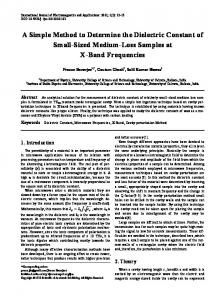
Cureton and Mulaik (1975) was used as the prerotated starting solution for this problem. The third data set is documented in Harman (1960), and goes back to studies of Holzinger. The subjects were 145 children in Chicago, who worked on 24 tests (for the labels of the tests, see Table 4). The fourth is the Ball-problem (Cattell & Dickman, 1962). This data set is based on 32 measures, as diameter and weight, taken from a sample of 80 balls. The fth data set is based on Overall and Kletts (1972) study of 6000 patients with 16 variables of the \Brief Psychiatric Rating Scale". The sixth data set is based on a study by Horn (1963), consisting of 172 male subjects. The subjects worked on items of the 16 P.F. and on some additional items. The seventh data set is a study of Baehr (1963), where 400 groups of subjects completed 30 items concerning their working situation. The eigth data set is based on Rimoldi's (1948) study of 138 subjects in 19 intelligence tests. The ninth data set is based on a study by Pemberton (1952) of 154 subjects with 25 tests. Criteria for comparison. For the empirical comparison of the solutions of different methods of oblique rotation, the following criteria are proposed: the number of main loadings is de ned as about a2 =h2 :50 (Furntratt, 1969), the hyperplane count without division of the absolute loadings by h, and the hyperplane count with division of the absolute loadings by h, and the number of factors with signi cant simple structure according to the test of Bargmann (1955). The solutions will not be compared with visually rotated solutions, because of the subjective component in visual rotation. Compared methods of factor rotation. The Trasid-rotation will be compared with Promax-, Oblimin- and Harris-Kaiser II-rotation. For the three methods, several parameters for the obliqueness of the solutions will be entered and the solution with the best hyperplane count (with division by h) will be retained. In addition, the published results for Maxplane-rotation and the few empirical results for Hyball-, PPFP-, Promaj- and Simplimax-rotation will be discussed. Comparison of the solutions. With respect to the number of main loadings according to Furntratt (1969) the Trasid-rotation should not be inferior. The number of main loadings are comparable for the dierent methods of factor rotation (see Table 1). For the Promax-solutions the mean value for the percent main loadings is slightly below the values of the remaining methods. For the mentioned new methods of factor rotation and for Maxplane, no values for the main loadings have been published. With regard to the hyperplane count, rst an illustration of the maximisation of the hyperplane count with division by h will be given. In Figure 3 the hyperplane count is plotted by the width W of Trasid-iterations. One can see that, with the exception of the data sets of Horn and Pemberton, no increase of the hyperplane counts occurs for a width greater than 0.10. On the whole, the increase of hyperplane counts is not important for the widths greater than 0.07. So, in the present data sets, a width of 0.15 seems sucient to reach an optimal simple structure. In cases with complex data and many factors (above 10) a greater width (e.g. 0.20) may be recommended. Trasid is expected to yield superior results for the hyperplane count in comparison to the other methods of factor rotation. The mean percentages for the hyperplane count (last row in Table 2) will be compared. The simple structure can be evaluated with regard to the hyperplane count without division by h (i.e. the number of variables with jaj 0:10) and for the hyperplane count with division by h (i.e. the number of variables with jaj=h 0:10). Concerning Maxplane only for values for the hyperplane count without division by h could be retained from Hakstian (1971). The Maxplane solutions have clearly the lowest values for the hyperplane count. Harris-Kaiser II-, Promax- and Oblimin-rotation yield comparable hyperplane counts. MPR{online 1997, Vol.2, No.2


125


Table 1:

Number of variables with

2

2

a =h

50 (Furntratt-criterion) :

Data set Factors H-K II Promax Oblimin Trasid Thurstone-20 3 20 (100) 20 (100) 20 (100) 20 (100) Thurstone-26 3 26 (100)* 24 (92) 26 (100)* 24 (92) Harman 4 24 (100) 22 (92) 22 (92) 22 (92) Cattell/Dickman 4 31 (97) 31 (97) 31 (97) 30 (94) Overall/Klett 4 16 (100) 16 (100) 16 (100) 16 (100) Horn 5 11 (55) 12 (60) 13 (65) 16 (80) Baehr 6 28 (93) 28 (93) 29 (97) 28 (93) Rimoldi 7 15 (79) 13 (68) 15 (79) 13 (68) Pemberton 8 22 (88) 18 (72) 20 (80) 21 (84) Mean 21 (89) 20 (86) 21 (89) 21 (89) Notes. The percent values are in brackets. They are refered to an optimum of one main loading for every variable. In the last row are the mean values for the nine (or eight) data sets. *These solutions correspond largely to the unrotated solutions after factor extraction (i.e. all main loadings on the rst factor) and are not included in the respective mean value.

Figure 3:

iteration

Plot of the hyperplane count with division by h by the width of the Trasid-




126

However, the Oblimin-solution have slightly higher hyperplane counts. The Trasidsolutions clearly have the highest number of variables falling in the hyperplane. This holds for the number of variables with jaj=h 0:10 as well as the number of variables with jaj 0:10. Not only is the mean percentage highest, but there is also no solution where Trasid yields a lower hyperplane count than any other method in Table 2. The data set with the 24 tests (Harman, 1960) has been analysed via PPFP (Katz & Rohlf, 1975). There were 46 absolute loadings 0.10, which is only one less than in the Trasid-solution and more than in the Maxplane-, Harris-Kaiser II-, Promax-, and Oblimin-solution (see Table 2). For Overall and Klett's (1972) data set, PPFP yields 31 absolute loadings 0.10 (see Katz & Rohlf, 1975), whereas Trasid yields 33 absolute loadings 0.10 (see Table 2). Harman's 24 tests have also been analysed via Simplimax-rotation (Kiers, 1994), where 40 absolute loadings with 0.10 resulted, which is less than with Trasid or PPFP. For the 26-variables Box-problem, there were 27 variables in the hyperplanes. This is exactly the value of the Promax- and Trasid-solution, but with the weighted Varimax-solution of Cureton and Mulaik (1975) as starting position, whereas Simplimax reaches it without this prerotation. However, Oblimin- and Harris Kaiser II-rotation do not reach this solution, even when starting from the weighted Varimax-solution. A comparison with the Hyball-procedure (Rozeboom, 1991b) was possible only for Harman's 24 tests. The best Hyball-variant (scan) reaches exactly the same number of variables with absolute loadings 0.10 as Trasid. Since there was no information about the absolute loadings divided by h, a comparison could not be made for this parameter. Another comparison with 10 factors out of a data set by Thurstone (1938) was not possible because Rozeboom (1991b) does not mention the method of factor extraction used. The third data set in Rozeboom (1991b) has not been published, consequently it could not be submitted to Trasid-rotation. The Promaj-rotation (Trenda lov, 1994) of Harman's 24 tests yields 40 variables in the hyperplane. This corresponds to the value of Simplimax and is clearly below the value of Trasid-, Hyball-, and PPFP-rotation. The Promaj-solution of the 20variables Box-problem has 20 variables in the hyperplane, which is below the value reached with Harris-Kaiser II-, Promax-, Oblimin- and Trasid-rotation (see Table 2). From this it may be concluded, that the Promaj-rotation might be an interesting method of factor rotation, but that it probably does not maximise the hyperplane count. While the Trasid-solutions have a higher mean hyperplane count than the Maxplane-, Harris-Kaiser II-, Promax-, and Oblimin-solutions, the dierence is quite small compared to PPFP. With the Hyball-rotation only one comparison resulting in an equal number of absolute loadings 0.10 was possible. In comparison to the Simplimax- and Promaj-solutions the Trasid-solutions have clearly more absolute loadings 0.10. The Trasid-rotation can also be compared with the Harris-Kaiser II-, Promax-, and Oblimin-rotation on the basis of the test for the signi cance of simple structure developed by Bargmann (1955). Because the Bargmann test is based on the absolute loadings divided by h, which are below or equal 0.10, and the number of absolute loadings divided by h is higher in the Trasid-solutions than in the Harris-Kaiser II-, Promax-, and Oblimin-solutions, a greater number of factors with signi cant simple structure is expected for the Trasid-solutions. In Table 3 the number of factors with signi cant simple structure according to Bargmann (1955) is shown for three dierent levels of signi cance. For all levels of signi cance the number of factors with signi cant simple structure is greater with Trasid, than with Harris-Kaiser II, Promax, and Oblimin. The dierences on the 25%-level are also relevant here, because the Bargmann test is MPR{online 1997, Vol.2, No.2



H{K II 27 (68)/ 27 (68) 7 (13)/ 7 (13)* 31 (43)/ 41 (57) 52 (54)/ 53 (55) 16 (33)/ 22 (46) 26 (33)/ 43 (54) 86 (57)/ 99 (66) 46 (40)/ 67 (59) 90 (51)/109 (62) 47 (47)/ 58 (58)

:

a

:

Maxplane Promax Oblimin / 25 (63) 27 (68)/ 27 (68) 27 (68)/ 27 (68) 27 (52)/ 27 (52) 11 (21)/ 11 (21)* / 32 (44) 32 (44)/ 39 (54) 31 (43)/ 40 (56) 65 (68)/ 67 (70) 67 (70)/ 68 (71) 18 (38)/ 25 (52) 19 (40)/ 27 (56) / 35 (44) 29 (36)/ 43 (54) 31 (39)/ 39 (49) 89 (59)/ 95 (63) 85 (57)/ 94 (63) / 45 (39) 52 (46)/ 67 (59) 55 (48)/ 72 (63) 91 (52)/113 (65) 91 (52)/115 (66) / 34 (48) 48 (51)/ 56 (60) 51 (52)/ 60 (62)

a =h

Hyperplane count ( j j 10, behind j j 10)

Trasid 27 (68)/ 27 (68) 27 (52)/ 27 (52) 43 (60)/ 47 (65) 77 (80)/ 78 (81) 29 (60)/ 33 (69) 48 (60)/ 52 (65) 109(73)/114 (76) 78 (68)/ 84 (74) 128(73)/129 (74) 63 (66)/ 66 (69)

a =h

:

a

:

Notes. The percent values are in brackets. They are refered to the maximum of variables in the hyperplane, based on the assumption of one main loading for every variable. Before the slash are the values for j j 10, behind for j j 10. In the last row are the mean values for the nine (or eight) data sets. *These solutions correspond largely to the unrotated solutions after factor extraction (i.e. all main loadings on the rst factor) and are not included in the respective mean value. For Thurstones 26-Variables problem Cureton and Mulaik's (1975) weighted Varimax solution was used as starting solution for Harris-Kaiser-, Promax-, Oblimin- and Trasid-Rotation.

Thurstone-20 Thurstone-26 Harman Cattell/Dickman Overall/Klett Horn Baehr Rimoldi Pemberton Mean

Table 2:


127


128


Table 3:

(1955)

Number of factors with signi cant simple structure according to Bargmann

Data set Harris-Kaiser II Promax Oblimin Trasid Thurstone-20 p .01 3 3 3 3 p .05 3 3 3 3 p .25 3 3 3 3 Thurstone-26 p .01 0 3 0 3 p .05 0 3 0 3 p .25 1 3 1 3 Harman p .01 1 2 0 3 p .05 1 2 1 3 p .25 3 2 3 4 Cattell/Dick p .01 2 3 4 4 p .05 3 3 4 4 p .25 3 4 4 4 Overall/Klett p .01 0 0 0 0 p .05 0 0 0 1 p .25 0 1 2 4 Horn p .01 0 0 0 2 p .05 0 0 0 3 p .25 0 1 1 4 Baehr p .01 3 3 3 5 p .05 4 4 4 5 p .25 4 5 6 6 Rimoldi p .01 0 0 0 2 p .05 0 0 0 3 p .25 1 1 0 6 Pemberton p .01 0 1 1 4 p .05 1 2 2 7 p .25 3 2 4 7 Sum p .01 9/ 9 15/12 11/11 26/23 p .05 12/12 17/14 14/14 32/29 p .25 18/17 22/19 24/23 41/38 Notes. The rst column contains the data sets and the levels of signi cance for simple strcture. In the following columns contain the number of factors with signigicant simple structure. In the last row the sum of factors with signi cant simple structure is reported. Behind the slash, the values are reported without the Thurstone-26 data set, because it could not be rotated with Oblimin and Harris-Kaiser II.



129

A new method for oblique rotation... Table 4:

Trasid-solution for 24 psychological tests (primary pattern)

Test F1 Verbal F2 Speed F3 Deduction F4 Memory Visual Perception -.02 .07 .70 .04 Cubes .01 -.02 .46 .01 Paper From Board .06 -.09 .59 -.03 Flags .10 -.02 .56 -.05 General Information .79 .07 .01 -.03 Paragraph Compreh. .79 -.08 .06 .05 Sentence Completion .89 .02 -.01 -.10 Word Classi cation .51 .13 .24 -.03 Word Meaning .86 -.19 .07 .09 Addition .07 .73 -.29 .23 Code .06 .58 -.10 .33 Counting Dots -.13 .73 .07 .07 Straight-Curved Cap. .04 .58 .27 -.04 Word Recognition .17 .05 -.03 .48 Number Recognition .04 -.05 .14 .48 Figure Recognition -.05 -.05 .45 .37 Object Number .05 .06 .02 .64 Number-Figure -.17 .15 .32 .51 Figure-Word .04 .04 .22 .35 Deduction .27 -.05 .45 .12 Numerical Puzzles .01 .30 .35 .17 Problem Reasoning .29 -.13 .40 .24 Series Completion .24 .06 .53 .07 Arithmetic Problems .26 .35 .07 .26 P jaj :10 12 14 9 12 P ja=hj :10 11 13 8 11 Correlations F1 1.00 among factors F2 .41 1.00 F3 .48 .46 1.00 F4 .35 .27 .26 1.00 Notes. The loadings :30 are printed in bold face. known to be conservative. The clear superiority of the Trasid-rotation in this criterion is probably due to the fact that the number of absolute loadings divided by h below or equal to 0.10 is maximised with the greatest priority with Trasid. For the new methods of factor rotation PPFP, Simplimax, Hyball, and Promaj no comparison could be drawn based on the Bargmann test, because no information on the number of absolute loadings divided by h lower than or equal to 0.10 has been reported. Because the Trasid-solutions have generally a very high hyperplane count, they may be dierent from many other solutions. So, it might be interesting to give an example in order to show if the solutions are just simpler derivates of the solutions that are generally reported in the literature or if they are substantially dierent. Because Harman's 24 tests are one of the most cited example, the factor pattern for this data set is reported here (see Table 4). The solution is quite close to the Oblimin-solution reported in Harman (1976, p. 324) or the Promax-solution reported in Hendrickson and White (1964). The main dierence is, that much more variables fall into the hyperplane in the Trasidsolution, but the meaning of the factors did not change. However, the intercorrelations of the factors are very dierent for the two solutions. This is, what was MPR{online 1997, Vol.2, No.2


130


Hyperplane count after maximising the number of absolute loadings .10 with Trasid-rotation exclusively

Table 5:

Thurstone-20 Thurstone-26 Harman Cattell/Dickman Overall/Klett Horn Baehr Rimoldi Pemberton Mean

a .10/ a/h .10 Bargmann-Test 27 (68)/ 27 (68) 3/3/3 26 (50)/ 27 (52) 2/3/3 21 (29)/ 51 (70) 0/0/2 70 (73)/ 79 (82) 4/4/4 13 (33)/ 36 (75) 0/0/1 24 (30)/ 59 (74) 0/0/1 85 (57)/119 (79) 3/5/5 43 (37)/ 88 (77) 0/0/0 94 (54)/138 (79) 1/2/4 45 (48)/ 69 (73) 13 / 17 / 23

Notes. In the second column, before the slash are the values for jaj=h :10, behind are the values for a :10. The percent values are in brackets. They are refered to an optimum of one main loading for every variable. The third column contains the number of factors with signi cant simple structure. Before the rst slash are the values for p :01, after the rst slash for p :05 and after the second slash for p :25. In the last row are the mean values for the nine (or eight) data sets.

observed in general, when Trasid-solutions were compared with other methods of factor rotation: The solutions dier often with regard to the intercorrelations of the factors, but less with regard to the main loadings in the factor pattern. The differences between the intercorrelations of the factors are especially important when factor solutions of higher order are intended. But also, when the intercorrelations among factors are interpreted in terms of the relations between constructs, these differences are very important. It should be noted that dierent cut-o values for the hyperplane and, more generally, dierent criteria for simple structure may produce dierent solutions. Trasid only attemps to yield optimal hyperplane counts.

2.4 Maximising the number of absolute loadings 0.10 only

Results with Trasid. The possibility of maximising only the number of absolute loadings 0.10 without division by h has already been mentioned. First, an example is given to demonstrate that a much higher number of absolute loadings 0.10 can be attained, if the number of absolute loadings divided by h lower than or equal to 0.10 is not maximised (see Table 5). The mean percentage hyperplane count is about 73% and higher than for the Trasid-rotation with priority in maximising the hyperplane count with division by h, where it was about 69%. The dierence between this and the other methods of factor rotation including Hyball-rotation is clear. However, also the number of absolute loadings divided by h falling in the hyperplane is still comparable with the values of the Harris-Kaiser II-rotation (see Table 2). So, when there is no restriction concerning the division of the loadings by h, the results are also very convincing. But the reduction of the number of factors with signi cant simple structure according to the Bargmann-test is very important. While the Trasid-rotation { which maximises the number of absolute loadings divided by h lower than or equal to 0.10 { yields 32 factors with signi cant simple structure on the 5%-level (see Table 3), there are only 17 factors with signi cant simple structure on the 5%-level, if maximisation is not based on the absolute loadings divided by h (see Table 5). This shows that the simple maximisation of the hyperplane count, without taking into MPR{online 1997, Vol.2, No.2


131


Example: Starting matrix with variables with moderate and low communality

Variable V1 V2 V3 V4 V5 V6 V7 V8 V9 V10 V11 V12 V13 V14 V15 V16 V17 V18 V19 V20 P

F1

F2 .60 .00 .60 .00 .60 .00 .00 .60 .00 .60 -.20 .00 -.20 .00 -.20 .00 -.20 .00 -.20 .00 -.20 .00 -.20 .00 -.20 .00 -.20 .00 -.20 .00 -.20 .00 -.20 .00 -.20 .00 -.20 .00 -.20 .00 j a j : 10 P ja=hj :10 22 18 18

F3 .00 .00 .00 .00 .00

.60 .60 .60 .60

h2

.36 .36 .36 .36 .36 .40 .40 .40 .40 .08 .08 .08 .08 .08 .08 .08 .08 .08 .08 .08 PP

-.20 -.20 -.20 -.20 -.20 -.20 -.20 -.20 -.20 -.20 -.20 5 PP 25 25 5

Notes. The main loadings are printed in bold face.

account the communalities of the variables, produces less convincing results in the Bargmann test. In addition, this example shows that a high number of absolute loadings lower than or equal to 0.10 does not guarantee a signi cant simple-structure according to the Bargmann test. This is a strong argument for the maximisation as it is proposed with Trasid-rotation, and it is also an argument against the tendency in the literature to report only the number of absolute loadings lower than or equal to 0.10 as an indicator for simple structure without taking into account the communality of the variables. Example: Trasid- and Oblimin-rotation with variables of low communality. Moreover, the question arises, to what extent do variables with low communality in uence the rotation, if not the hyperplane count based on the loadings divided by h but the simple hyperplane count is maximised. In order to examine this question, a matrix with 9 variables of moderate communality (.36-.40) and 11 variables of very low communality (.08) was constructed (see Table 6). The variables with moderate communality all clearly load on one of the three factors. Some of them have secondary loadings, which may fall into the hyperplane after oblique rotation. But also the loadings of variables with low communality may fall into the hyperplane after oblique rotation. The number of absolute loadings 0.10 and absolute loadings divided by h 0:10 is equal in this matrix. Now, it can be examined how the orientation on the loadings with or without division by h, in uences the rotation. First, a direct Oblimin solution (with delta=0) is reported (see Table 7). In the starting solution the number of absolute loadings 0.10 was 25. In the Oblimin-solution the number of absolute loadings 0.10 is 33. But the number of MPR{online 1997, Vol.2, No.2


132


Table 7:

Example: Oblimin-solution with variables with moderate and low communality

F2 F3 h2 .52 .00 -.37 .36 .52 .00 -.37 .36 .52 .00 -.37 .36 .00 .60 .00 .36 .00 .60 .00 .36 .13 .00 .60 .40 .13 .00 .60 .40 .13 .00 .60 .40 .13 .00 .60 .40 -.28 .00 -.04 .08 -.28 .00 -.04 .08 -.28 .00 -.04 .08 -.28 .00 -.04 .08 -.28 .00 -.04 .08 -.28 .00 -.04 .08 -.28 .00 -.04 .08 -.28 .00 -.04 .08 -.28 .00 -.04 .08 -.28 .00 -.04 .08 -.28 .00 -.04 PP .08 j a j : 10 2 18 13 P ja=hj :10 2 18 2 PP 33 22 Variable V1 V2 V3 V4 V5 V6 V7 V8 V9 V10 V11 V12 V13 V14 V15 V16 V17 V18 V19 V20 P

F1

Notes. The loadings greater than .40 are printed in bold face. The intercorrelations of the factors are in Tabelle 8.



133


Example: Trasid-solutions with variables with moderate and low communality

Variable V1 V2 V3 V4 V5 V6 V7 V8 V9 V10 V11 V12 V13 V14 V15 V16 V17 V18 V19 V20 P

F1

.59 .59 .59

.03 .03 .04 .04 .04 .04 -.28 -.28 -.28 -.28 -.28 -.28 -.28 -.28 -.28 -.28 -.28 j a j : 10 P ja=hj :10 66

Trasid1 F2 F3 .04 -.41 .04 -.41 .04 -.41 .60 .03 .60 .03 -.05 .62 -.05 .62 -.05 .62 -.05 .62 .00 -.02 .00 -.02 .00 -.02 .00 -.02 .00 -.02 .00 -.02 .00 -.02 .00 -.02 .00 -.02 .00 -.02 .00 -.02 18 13 18 13

Trasid2 F2 F3 .56 .09 -.28 .56 .09 -.28 .56 .09 -.28 .08 .63 -.07 .08 .63 -.07 .05 -.09 .64 .05 -.09 .64 .05 -.09 .64 .05 -.09 .64 -.27 -.01 -.09 -.27 -.01 -.09 -.27 -.01 -.09 -.27 -.01 -.09 -.27 -.01 -.09 -.27 -.01 -.09 -.27 -.01 -.09 -.27 -.01 -.09 -.27 -.01 -.09 -.27 -.01 -.09 -.27 -.01 -.09 6 18 13 4 11 0 F1

h2

.36 .36 .36 .36 .36 .40 .40 .40 .40 .08 .08 .08 .08 .08 .08 .08 .08 .08 .08 .08

Notes. The loadings greater than .40 are printed in bold face. The intercorrelations of the factors are in Tabelle 8.

loadings divided by h fell from 25 to 22. The most important change is in factor F3. The secondary loadings of the variables V10 to V18 are now -.04. When this loadings are divided by h they are .14 and do not fall into the hyperplane. Note that in factor F1 four loadings of the variables V6 to V9 (which have the highest communality in this example) do not fall into the hyperplane. In Table 8 two Trasid-solutions (after Varimax-prerotation, as described above) are presented, the rst (Trasid1, left side) is based on the above-mentioned algorithm with highest priority for the maximisation of the absolute loadings divided by h lower than or equal to 0.10. For the second solution (Trasid2, right side) the Trasid-algorithm only maximises the number of absolute loadings 0.10. In the second Trasid-solution maximising the absolute loadings 0.10 (without division by h) with highest priority, there are 37 absolute loadings 0.10, which is more than in the Oblimin-solution. However, there are only 15 absolute loadings divided by h, which are lower than or equal to 0.10, compared to 22 in the Oblimin solution. In both solutions the number of absolute loadings 0.10 has been maximised, whereas the number of absolute loadings divided by h lower than or equal to 0.10 was reduced. Because the number of loadings 0.10 was also maximised in the variables with low communality (.08), both solutions have been in uenced by those variables. The rst Trasid-solution (Trasid1, see Table 8) diers clearly from the Obliminsolution and the second Trasid-solution. The number of absolute loadings (both divided by h and not divided by h) which are lower than or equal to 0.10 is 37 in both cases and has been maximised. The variables with low communality have also MPR{online 1997, Vol.2, No.2


134


solutions

Intercorrelations of the factors for the Oblimin-solution and the two Trasid-

Trasid1 Trasid2 Oblimin -.08 -.21 .00 .32 .01 .03 .25 .12 .00 a little in uence on the solution, which can be seen in the fact that the absolute loadings of variables with low communality (V1 to V11), which were above 0.10 in the starting solution, are now below 0.10 for the factor F3. But the most important fact is, that the hyperplane count divided by h is maximal for all the variables with high communality (V1 to V9), which is not the case in the Oblimin- and in the second Trasid-solution. In fact, in Trasid2 only four loadings of the variables with high communality (V6 to V9 on F1) fall into the hyperplane with division by h, in Oblimin the loadings of V6 to V9 on F1 do not fall into the hyperplane at all. However, both in the Trasid1-solution and in the Oblimin-solution the secondary loadings of the variables V1 to V3 are high, which is not so much the case in the Trasid2-solution. This may be an interesting aspect of the Trasid2-solution. But, as mentioned above, the \true" complexity of the variables V1 to V3 is not known, so that this point needs further exploration. But since it is related to the medium loadings, it is not directly related to the hyperplane count and is therefore not treated here. All in all, it should not be excluded that Trasid2 yields interesting solutions, but the hyperplane count with division by h will in most cases probably not be maximal for the variables with high communality. The dierences in the maximisation of the absolute loadings 0.10 with division by h leads also to very dierent intercorrelations of the factors (see Table 9). The fact that the intercorrelations between the Oblimin-factors are very dierent from those of the other solutions is not very surprising, because the Obliminsolution diers from the other two solutions with regard to the hyperplane count (both with and without division by h). But it is interesting to note, that in the second Trasid-solution, there are 37 absolute loadings 0.10 (without division by h), whereas in the Oblimin solution there are 33. The dierence of 4 variables in the hyperplane count (without division by h) is accompanied by important dierences in the intercorrelations of the factors. This corresponds to Cattell's (1988) opinion that slight dierences in the hyperplane count may lead to important dierences between factor solutions. However, the second Trasid-solution has the same number of absolute loadings 0.10 without division by h as the rst Trasid-solution (i.e. 37, see Table 8). But the intercorrelations between the factors are very dierent for the two Trasid-solutions. Thus, the dierence between the solutions with regard to the number of absolute loadings 0.10 with division by h (15 versus 37, see Table 8) is important with regard to the intercorrelations of factors. Maximising the number of absolute loadings 0.10 without division by h may lead to factor intercorrelations very dierent from those, which are obtained, when the number of absolute loadings 0.10 with division by h is maximised with the highest priority. In the case that there are many variables with low communality and if only the number of absolute loadings 0.10 without division by h is maximised, the maximisation of the hyperplane count may be primarily due to variables with low communality. In this sense, an in uence of variables with low communality on the Oblimin- and Trasid2-solutions could be shown, which means that Oblimin- and Trasid2-solutions have to be regarded with caution, when they are based on data sets with many variables with low communality. MPR{online 1997, Vol.2, No.2



135

3 Discussion In an empirical comparison, the new method of factor rotation called Trasid has been shown to yield solutions with more optimal simple structure than Harris-Kaiser II-, Promax-, and Oblimin-rotations with regard to the hyperplane count. Especially the number of factors with signi cant simple structure according to Bargmann (1955) is nearly double those in the Trasid-solutions compared to the Harris-Kaiser II-, Promax-, and Oblimin-solutions. Some empirical comparisons with new methods of oblique factor rotation as PPFP-, Simplimax-, and Promaj yield lower hyperplane counts for these methods. For the Hyball-rotation only one comparison was possible for Harman's 24 tests, which yields the same number of absolute loadings 0.10. Further comparisons are necessary. When the number of absolute loadings 0.10 without divison by h is maximised with priority, the hyperplane count is even higher in the Trasid-solution than in the Hyball-solution. But it could be shown that maximising of absolute loadings 0.10 without division by h does not maximise the number of factors with signi cant simple structure according to Bargmann (1955). It could be demonstrated in an example, that simple structure should not be maximised only with regard to the number of absolute loadings 0.10, if an in uence of variables with low communality on the solution is to be avoided. Oblimin-rotation may also be in uenced by variables with low communality. This point is important because variables with low communality are often variables with low reliability. Maximising hyperplane counts or maximising simple structure in general may be problematic, if the simple structure is maximised on the basis of the variables with the lowest reliability in a data set. Additional studies on the in uence of variables with low communalities on rotation with dierent methods of factor rotation are necessary. There may be dierent ways to deal with this problem, but Trasid-rotation is at least one way to avoid the diculties with variables of low communality and possibly low reliability. It should be noted, that direct maximisation of the hyperplane count may have some correspondence with the treatment of factor loadings in con rmatory factor analysis: non-signi cant loadings and loadings which are expected to be nonsigni cant are generally xed as zero-elements in the factor matrix. This means that in the context of con rmatory factor analysis, the factor matrix is rarely forced to correspond to a complex criterion of analytical factor rotation as for example the Varimax- or Oblimin-criterion. In most cases of con rmatory factor analysis, only signi cant and non-signi cant loadings are dierentiated. Thus, a method of factor rotation like Trasid, which focusses only on main loadings and on maximisation of zero-elements instead of maximising a complex analytical criterion is closer to the treatment of the loadings in con rmatory factor analysis. So, results of con rmatory and exploratory factor analysis can more easily be compared, if Trasid-rotation is used for rotation in the exploratory context. Even in the case, that one wants to identify the maximum of zero-elements in exploratory factor analysis via oblique rotation before xing them to zero in con rmatory factor analysis, Trasid-rotation may be recommended. The above-mentioned problem of maximising zero-elements in factor matrices, which may be due to unreliability of the variables, is also important in the case of con rmatory factor analysis, but this issue cannot be dealt with here. More generally, the following can be concluded: if an oblique simple structure is intended, and if one wants to maximise the hyperplane count of a solution, the Trasid-rotation can be recommended. In addition, Trasid-rotation helps to avoid the in uence of variables with low communality on factor rotation. A programme for PC (DOS) enabling Trasid-rotation with up to 20 factors is available on request from the author. MPR{online 1997, Vol.2, No.2



136

References

[1] Baehr, M.E. (1963). A comparison of graphic and analytic solutions for both oblique and orthogonal simple structures for factors of employee morale. Psychometrika, 28, No. 2, 199-209. [2] Bargmann, R. (1955). Signi kanzuntersuchungen der einfachen Struktur in der Faktoren-Analyse. Mittbl. math. Statist., 7, 1-24. [3] Beauducel, A. (1996). Zur Optimierung der schiefwinkligen Rotation zur Einfachstruktur durch Berucksichtigung der faktoriellen Komplexitat von Variablen. In Unvero. Diss., Freie Universitat Berlin, FB Erziehungswissenschaft, Psychologie und Sportwissenschaft (Hrsg.). [4] Boyle, G.J. & Stanley, G.V. (1986). Application of factor analysis in psychological research: Improvement of simple structure by computer-assisted graphic oblique transformation: A brief note. Multivariate Experimental Clinical Research, 8, 175-182. [5] Burdsal, C. & Bolton, B. (1979). An item factoring of 16PF-E: Further evidence concerning Cattell's normal personality sphere. Journal of General Psychology, 100, 103-109. [6] Carroll, J.B. (1957). Biquartimin criterion for rotation to oblique simple structure in factor analysis. Science, 125, 1114-1115. [7] Cattell, R.B. (1952). Factor analysis: an introduction and manual for the psychologist and social scientist. New York: Harper. [8] Cattell, R.B. (1988). The meaning and strategic use of factor analysis. In J.R. Nesselroade & R.B. Cattell (Hrsg.), Handbook of multivariate experimental psychology (2nd Edition) (S. 131-201). New York: Plenum Press. [9] Cattell, R.B. (1994). Constancy of global, second-order personality factors over a twenty-year-plus period. Psychological Reports, 75, 3-9. [10] Cattell, R.B. & Dickman, K.W. (1962). A dynamic model of physical in uences demonstrating the necessity of oblique simple structure. Psychological Bulletin, 59, 389-400. [11] Cattell, R.B. & Muerle, J.L. (1960). The \Maxplane" program for factor rotation to oblique simple structure (Bd. 20, S. 569-590). [12] Cureton, E.E. & Mulaik, S.A. (1975). The weighted Varimax rotation and the Promax rotation. Psychometrika, 40, No. 2, 183-195. [13] Eber, H.W. (1966). Toward oblique simple structure: maxplane. Multivariate Behavioral Research, 1, 112-125. [14] Furntratt, E. (1969). Zur Bestimmung der Anzahl interpretierbarer gemeinsamer Faktoren in Faktorenanalysen psychologischer Daten. Diagnostica, 15, 62-75. [15] Gorsuch, R.L. (1970). A comparison of Biquartimin, Maxplane, Promax, and Varimax. Educational and Psychological Measurement, 30, 861-872. [16] Gorsuch, R.L. (1983). Factor Analysis. Hillsdale, NJ: Lawrence Erlbaum. [17] Hakstian, A.R. (1971). A comparative evaluation of several prominent methods of oblique factor transformation. Psychometrika, 36, No. 2, 175-193. [18] Hakstian, A.R. & Abell, R.A. (1974). A further comparison of oblique factor transformation methods. Psychometrika, 39, No. 4, 429-444. [19] Hakstian, A.R. & Boyd, W.M. (1972). An empirical investigation of some special cases of the general \Orthomax" criterion for orthogonal factor transformation. Educational and Psychological Measurement, 32, 3-22. [20] Harman, H.H. (1960). Modern factor analysis. Chicago: The University of Chicago Press. [21] Harman, H.H. (1976). Modern factor analysis. Chicago: The University of Chicago Press. MPR{online 1997, Vol.2, No.2



137

[22] Harris, C.W. & Kaiser, H.F. (1964). Oblique factor analytic solutions by orthogonal transformations. Psychometrika, 29, 347-362. [23] Hendrickson, A.E. & White, P.O. (1964). Promax: a quick method for rotation to oblique simple structure. The British Journal of Statistical Psychology, 17, Part 1, 65-70. [24] Hochhausen, R. (1976). Untersuchungen im Rahmen des Forschungsprojektschwerpunktes \Produktives Denken und Problemlosen": B) Versuche zur Operationalisierung objektiver und subjektiver Komplexitat. Unveroentlichte Diplomarbeit. Freie Universitat Berlin, Fachbereich Erziehungs- und Unterrichtswissenschaften, Institut fur Psychologie. [25] Horn, J. (1963). Second-order factors in questionnaire data. Educational and Psychological Measurement, 23, No. 1, 117-134. [26] Jennrich, R.I. & Sampson, P.F. (1966). Rotation for simple loadings. Psychometrika, 31, 313-323. [27] Kaiser, H.F. (1958). The varimax criterion for analytic rotation in factor analysis. Psychometrika, 23, 187-200. [28] Kaiser, H.F. & Cerny, B.A. (1978). Casey's method for tting hyperplanes from an intermediate orthomax solution (Multivariate Behavioral Research (13:, 395-401. [29] Katz, J.O. & Rohlf, F.J. (1974). Functionplane { a new approach to simple structure rotation. Psychometrika, 39, No. 1, 37-51. [30] Katz, J.O. & Rohlf, F.J. (1975). Primary product functionplane: An oblique rotation to simple structure (Bd. 10, S. 219-232). In Multivariate Behavioral Research (Hrsg.). [31] Kiers, H.A.L. (1994). Simplimax: Oblique rotation to an optimal target with simple structure. Psychometrika, 59, 567-579. [32] Marshall, A.W. & Olkin, I. (1979). Inequalities: Theory of majorization and itsapplications. New York: Academic Press. [33] Overall, J.E. & Klett, C.J. (1972). Applied multivariate analysis. New York: McGrawHill. [34] Pawlik, K. (1967). Dimensionen des Verhaltens. Eine Einfuhrung in die Methodik und Ergebnisse faktorenanalytischer psychologischer Forschung. Bern: Hans Huber. [35] Piaggio, L. (1972). Modi kation des Promax-Verfahrens. Zeitschrift fur experimentelle und angewandte Psychologie, 19, 580-592. [36] Rimoldi, H.J. (1948). Study of some factors related to intelligence. Psychometrika, 13, No. 1, 27-46. [37] Rozeboom, W.W. (1991a). Hyball: A method for subspace-constrained factor rotation. Multivariate Behavioral Research, 26, 163-177. [38] Rozeboom, W.W. (1991b). Theory & practice of analytic hyperplane optimization. Multivariate Behavioral Research, 26, 179-197. [39] Rozeboom, W.W. (1992). The glory of suboptimal factor rotation: Why local minima in analytic optimization of simple structure are more blessing than curse. Multivariate Behavioral Research, 27, 585-599. [40] SAS (1982). User's guide: Statistics. Cary, NC: SAS Institute Inc. SPSS/PC+ (1988). Advanced statistics V 2.0. Chicago, Il: SPSS Inc. [41] Thurstone, L.L. (1947). Multiple factor analysis. Chicago: University of Chicago Press. [42] Trenda lov, N.T. (1994). A simple method for procrustian rotation in factor analysis using majorization theory. Multivariate Behavioral Research, 29, No. 4, 385-408. [43] Warburton, F.W. (1963). Analytic methods of factor rotation. The British Journal of Statistical Psychology, 16, 165-174. [44] Wittmann, W.W. & Hampel, R. (1976). Faktorenanalyse, Rotationsproblem und Implikationen fur die Testkonstruktion. Archiv fur Psychologie, 128, 219-239. MPR{online 1997, Vol.2, No.2



138

4 Acknowledgments I should like to express my gratitude to A.O. Jager and W.W. Wittmann for their supervision of my doctoral thesis, which contains preliminary work for this study. In addition, I am grateful to M. Kersting for helpful comments.

