electromagnetic energy from the transmitter toward the receiver. .... diffuse reflections from the rough surfaces (the fields reflected out of the specular ... of observation is sufficiently far removed from the surface to regard the scattered waves as.
A New Microcellular Propagation Model Based on Uniform Theory of Diffraction and Physical Optics Abstract: This paper introduces a deterministic propagation prediction model to predict the path loss in arbitrary-structured urban mobile radio environments. It uses a ray tracing technique to model the flow of electromagnetic energy from the transmitter toward the receiver. The image method is applied to trace the rays and the ray launching method is used to account for scattered fields. Analytical bases for calculating field contributions due to the rays are geometrical optics (GO) and uniform theory of diffraction (UTD), whereas physical optics (PO) is applied to estimate the contribution of scattered fields. In order to expedite the ray tracing process, a new ray tracing acceleration technique has been developed, which improves efficiency of the model in terms of reduced memory and CPU time requirements. It can also be incorporated with any ray propagation model. The predicted path loss results are compared with the measured data. Root mean square (rms) deviations from measurements are less than 4 dB for different line-of-sight (LOS) and non-line-of-sight (NLOS) routes.
1. Introduction Exact prediction of radio wave propagation characteristics in micro and picocells is rendered by applying the deterministic propagation prediction models, which are also known as sitespecific models [1]. Using deterministic models, the received field strength and power-delay profile (PDP) are predicted at different observation points regardless of complexity the scenario. Most of the deterministic models are based on the ray tracing methods and use the faceted models in order to model the geometry and morphology of the urban or indoor scenes. Ray propagation models can be classified into two main groups with respect to their strategy to trace the rays: techniques based on the shooting and bouncing rays (SBR) method [2] and techniques based on the image method [3]. In order to improve efficiency of the tedious ray tracing process, ray tracing acceleration techniques have been proposed. Most popular ray tracing acceleration techniques in literature are the binary space partitioning (BSP) [4], the space volumetric partitioning (SVP) [5], the angular z-buffer (AZB) [6], and the polar sweep [7] techniques. In this paper, a deterministic ray propagation model is presented. This model assumes major propagation mechanisms as line of sight (LOS) propagation, reflection, diffraction, and scattering. Moreover, a new ray tracing acceleration technique is developed and incorporated with the model.
2. Model Description The model assumes the received field as complex vector summation of following contributions: 1) direct (LOS) component; 2) single reflected and single diffracted rays;
1
3) rays due to double effects (double reflected, double diffracted, reflected-diffracted, and diffracted-reflected rays); 4) rays due to triple effects excluding triple diffracted rays; 5) scattered fields by ground or building surfaces. Contributions of the rays (categories 1 to 4) are evaluated by applying the geometrical optics (GO) and uniform theory of diffraction (UTD). The physical optics (PO) is applied to estimate contributions of the scattered fields.
2.1 – Ray Contributions The electric field for the direct component, LOS cases, with free space loss assumption is given by e jkd (1) ELOS E0 d The electric field for a single reflected ray is also given by jk s s e (2) ER E0 R s s and for a single diffracted ray by E s jk s s ED 0 D e (3) s s s s where wave number; k E0 emitted electric field; propagation path length; d s path length from the source to the reflection or diffraction point; path length from the reflection or diffraction point to the receiver; s Fresnel dyadic reflection coefficient; R D dyadic non-perfectly conducting wedge diffraction coefficient, as given in [8]. To evaluate other ray contributions arising from multiple effects such as multiple reflections, multiple diffractions, and multiple reflections-diffractions, appropriate combinations of the abovementioned formulas are applied. Moreover, for the special case of double diffractions by two consecutive wedges, higher-order diffracted fields are taken into account. In such cases, considering only first-order diffracted fields do not result in an accurate prediction [9]. Since the ground and walls are rough at mobile communications operating frequencies, their corresponding surface roughness attenuation factor is used to modify the Fresnel reflection coefficients. Consequently, the specularly reflected and diffracted fields can more precisely be estimated [10].
2.2 – Contribution of the Scattering Scattering mechanism is introduced in order to account for the electromagnetic energy that arrives at the receiver when the location of the transmitter, the receiver, and a surface do not fulfill the Snell’s law of reflection. Indeed, the scattering phenomenon is representative of the diffuse reflections from the rough surfaces (the fields reflected out of the specular direction). Thus, for a fixed transmission-reception geometry, the PO method is applied to evaluate contribution of the scattering phenomenon for those surfaces that the GO and UTD approach results in zero received field. The single scattered electric field component is calculated via
2
EPO
where k E0 s s i s s Lx , Ly R and
jk s s jke cos i 1 R cos s 1 R E0 4s s Ly L Lx Ly sinc k sin i sin s cos s x sinc k sin s sin s 2 2
(4)
wave number; emitted electric field; propagation path length from the transmitter to the scattering point; propagation path length from the scattering point to the receiver; angle of incidence; vertical scattering angle; horizontal scattering angle; scattering aperture dimensions; Fresnel dyadic reflection coefficient;
sin x . x The above expression is extracted using the Helmholtz integral and the Kirchhoff or PO approximation for a smooth rectangular aperture [11]. The geometry of scattering is depicted in Figure 1. A basic assumption, under which the scattered field given by (4) is valid, is that the point of observation is sufficiently far removed from the surface to regard the scattered waves as plane. Hence, the receiver should be placed at a distance of at least 2D2/λ, where D is the largest dimension of the scattering aperture [12]. Due to the multiplicative dependence of the scattered field from the propagation path lengths s and s , the magnitude of the received field takes very small values. Hence, it is useless to calculate double scattering or any combination with other propagation mechanisms in the propagation prediction model. The inclusion of scattering is vital especially in non-line-of-sight (NLOS) cases, where scattering and diffraction are the main propagation contributions. Furthermore, in LOS cases and urban sites, where the streets do not form a rectilinear grid and the buildings are not parallelepipeds erected along street sides, scattering contributes to the representation of the fading phenomenon. In order to estimate the scattered field components, the ray launching method is applied. Notice that the ray tracing process for evaluating the other components (rays of section 2.1) is accomplished using the image method. Ray launching at the transmitter is based on the technique proposed in [2], where a sinc x
z
Rx
Ly/2
Tx
E0v Lx/2
y EPOv
EPOh
i s
s
E0h
x Lx/2
Ly/2 Figure 1: Scattering geometry
3
regular icosahedron is inscribed in a unit sphere surrounding the transmitting antenna. Using this technique, we ensure that there is constant angular separation between rays, and each ray represents an equal and unique portion of the total spherical wavefront. For the scattering mechanism, the wavefront area of the ray under inspection determines the aperture size used for the calculation of the scattered field. The linear dimension of the wavefront area at a distance R from the source is approximately given by 4 (5) s R A where A is the number of launched rays.
2.3 – Total received electric field The total received electric field is calculated by complex vector addition of all field components arriving at the receiving antenna: (6) ETotal ELOS EGO EUTD EPO where the constituents ELOS , EGO EUTD , and EPO are representative of the direct (LOS) component, the ray contributions, and the contribution of the scattered fields, respectively. A complex vector addition of the received contributions enables us to observe the multipath interference and the rotation of the polarization vector due to different propagation mechanisms. The path loss is calculated by ETotal L 20log10 (7) 4 E 0 where E0 is again the emitted field strength.
3. Ray Tracing Acceleration In order to develop a practical propagation prediction model, it is necessary to utilize a suitable ray tracing acceleration technique that reduces number of the shadowing and rayobject intersection tests to save the memory and CPU time. Here, we propose a new ray tracing acceleration technique. This technique was inspired by the AZB technique and developed based on the SVP technique and the painter’s algorithm [13]. It aggregates advantages of both AZB and SVP techniques, whereas it is not as complex as the AZB technique. A detailed description of the technique is given in this section.
3.1 – Visibility Database As the beginning stage of the ray tracing process, the ray tracing acceleration technique receives the geometrical information of the scene as an input and returns the visibility database, which stores the visibility relationships among the transmitter and objects (facets and edges) of the environment. The database has a layered hierarchical structure, as shown in Figure 2. The first layer contains facets/edges, which are visible from the transmitter antenna. The transmitter illuminates these facets/edges directly. The subsequent layers are organized into groups of facets/edges that each group hangs on a facet/edge of the prior layer. The second layer includes facets/edges, which can take part in a second-order propagation mechanism together with a facet/edge of the first layer. In this order, the third layer includes facets and edges, which can take part in a third-order effect together with the related facet/edge of the second layer and its corresponding facet/edge in the first layer. The succeeding layers follow the same logic.
4
Layer1
Layer2
Layer3
Facet Facet
Facet Facet
Facet Edge Edge
Facet Edge Edge
Edge
Edge
Edge
Facet Facet
Facet Facet
Edge
Facet Edge Edge
Facet Edge Edge
Edge
Edge
Facet Facet
Facet Facet
Facet Edge Edge
Facet Edge Edge
Edge
Edge
Facet Facet
Facet Edge
Figure 2: Illustration of the hierarchical structure of the visibility database considering three visibility layers.
Three essential tools, used by the new ray tracing acceleration technique, are the SVP technique, the back-face culling [1], and the painter’s algorithm. Moreover, three layers for the visibility database are considered that can support the rays of section 2.1. In order to produce the visibility database, all facets/edges of the environment are assumed as potential reflectors and diffracting edges. Then, facets/edges, which are totally shadowed by other facets or situated outside of the relevant reflection or diffraction space, are discarded. Finally, only facets/edges that can take part in the desired propagation mechanisms (see section 2.1) are stored in the visibility database. To compose the first visibility layer, all facets/edges of the environment are subjected to consider. Applying the back-face culling and painter’s algorithm, facets/edges not illuminated by the source point (transmitter antenna) are sifted out and discarded. Ordering of the facets in terms of distance from the source point is maintained. Facets/edges that have been situated inside the reflection/diffraction space of each facet/edge of the first layer are nominated to be stored in the second layer. After determining these facets/edges, the back-face culling and the painter’s algorithms are applied to discard ones that are not illuminated by the source point of the reflection/diffraction space. As stated before, the subsequent layers can be composed following the same logic. A reflection space’s source is the well-known image source, which is determined applying the image theory, whereas a diffraction space’s source can be any point on the diffracting edge [14].
5
Reflection Space
Image Source
Image Source
Point Source
(a)
Point Source (b)
Figure 3: Illustration of the reflection space geometry: (a) Three dimensional geometry of the reflection space of a facet; (b) Two dimensional top view of the reflection space of a facet.
To determine facets/edges inside a reflection space, the geometry of the reflection space is specified in terms of the facet and the corresponding image source. The voxels totally or partially occupied by the space are determined. Subsequently, facets/edges stored in these voxels are taken as the reflection space’s facets/edges. The geometry of a typical reflection space is depicted in Figure 3. The geometry for a diffraction space is also specified in terms of the edge and the source that illuminates the edge. Figure 4 shows an example for the geometry of diffraction space. The voxels occupied by the space are determined and a similar procedure as described for a reflection space is followed.
3.2 – Shadowing Test In the ray tracing process, each ray category of section 2.1 is investigated considering the information of the visibility database. For example, in order to specify diffracted-reflected rays, only edges stored in the first visibility layer together with their corresponding facets in the second layer are inspected. During the ray tracing process, depending on the order of mechanism under consideration, the shadowing test can be performed up to four times for each ray. In the ray tracing world, shadowing test is known as the operation to determine if an observation point is visible from a source point. In other words, the shadowing test determines if any object of the scene occludes a given ray path from a source point to an Diffraction Space Diffracting Edge (b)
(a)
Point Source Diffraction Space
Point Source
(c)
Point Source
Figure 4: Illustration of the diffraction space geometry: (a) Three dimensional geometry of the diffraction space of an edge; (b) Two dimensional top view of the diffraction space of a vertical edge; (c) Two dimensional top view of the diffraction space of a horizontal edge.
6
observer point. In faceted models, the shadowing test is reduced to repeatedly applied rayfacet intersection tests. Apart from producing the visibility database, another duty of a ray tracing acceleration technique is to expedite the shadowing tests by minimizing the number of required ray-object intersection tests. The shadowing test is performed in the following fashion: given a ray with known source and observation points, the voxels pierced by the ray are distinguished. This can be done efficiently by incremental calculation when spatial partitioning is uniform [5]. Only facets stored in these voxels and visible from the source of the ray (considering the information of the visibility database) are tested for intersection. In the shadowing test, it is necessary to determine the closest facet pierced by the ray. An important observation is that the ray imposes a strict ordering on the pierced voxels from the voxel that contains the source to the voxel of the observer. This ordering guarantees that all intersections occurring in one voxel are closer to the ray origin than those in all subsequent voxels. Moreover, owing to the fact that closer facets can occupy wider solid angles, they can obstruct the ray path with a higher probability. Therefore, by processing the voxels in order in which they are encountered along the ray, it is not necessary to process the subsequent voxels once a ray-facet intersection has been found.
4. Simulation Results and Comparison with Measurements We chose two parts of Athens city center as the test areas, for which the measurement data have been presented in [15], [16]. Figure 5 depicts the plan views of these areas. The average building height in these parts of Athens is 15-20 meters [16]. The sampling rate for the measurement have been /10 while in the simulation, the computing step was 6 . These rates were used for plotting the respective curves. In Figure 6, we present a comparison between calculated results by the new model and by Kanatas et al. presented in [16] along with the measured path loss. The path loss is plotted versus distance between the base station (BS) and the mobile station (MS), for a case where the BS antenna is located at a height of 12.5 m and close to the street side, and the MS moves along the same street. For this case, Kanatas et al. have adopted a simple geometry model with high surrounding buildings and no crossroads. They have applied this approximation because the case is a LOS situation [16]. Another comparison is presented in Figure 7 for a case where the BS antenna is located at a height of 8.5 m and is at a distance of 2 m from the street side, as shown in the geometry plan view of Figure 5(a). The MS moves along the first parallel street. The building B1 (marked in Figure 5(a)) involves some anomalies, so we manipulated the original geometry presented in [16] in order to modify it. Consequently, the gap between the measured curve and the simulated one by Kanatas et al. up to a distance of 80 m in Figure 7 does not exist between the measured curve and the simulated one by the new model. Finally, Figure 8 shows a comparison between computed and measured path loss when the BS antenna is located at a height of 9 m in the middle of a street and the MS moves along a perpendicular street (see Figure 5(b)). In Figure 8, the simulated results by both the new model and Kanatas et al. are presented. In the simulation, the geometry of Figure 5(b) has been modified considering the anomalies of building block B2 (marked in Figure 5(b)). Root mean square (rms) deviations from measurements for the results of Figures 6-8 are represented in Table 1. Table 1: RMS Deviation from Measurements for the Results of Figures 7-9 New Model
Kanatas et al. [16]
LOS situation (Figure 6)
3.6 dB
7.2 dB
MS move in parallel street (Figure 7)
3 dB
6.2 dB
MS moves in perpendicular street (Figure 8)
3.1 dB
7 dB
7
10
10
10 30
10
Tx 30
10
Rx2
Rx1 7 50
B1
30
100
45
4 5
(a) 10
10
10
80
20
Rx2
Rx1 B2
60
20
Tx
85
80
75
40
80
(b)
Figure 5: Geometry plan views of the test areas.
Examining Figures 6-8, one can conclude that the new model provides more accurate predictions. The CPU time consumed to obtain the results of Figure 7 was only a few seconds using the new model, whereas using a mere SVP algorithm, it was about 3 minutes and using the AZB algorithm, it was about 25 seconds. The computing platform used for the simulation was a PC with an AMD-Athlon CPU operating at 1.333 GHz and 256 Mbytes of RAM.
5. Conclusion A new deterministic propagating model for predicting the path loss in urban microcellular mobile environments was developed. The model applies GO, UTD, and PO. A new ray tracing acceleration technique was also proposed, which can efficiently mitigate computational burden of the ray tracing process. This technique can be easily implemented and incorporated with any ray propagation model. The new model imposes no limitation on the geometrical structure of the environment. In other words, the model can suitably handle irregular terrain and buildings configurations. Moreover, it takes into account the diffuse reflections as the scattering mechanism as well as the influence of surface roughness on the specular reflections.
8
-50
-60
New Model Kanatas et al. [16] [22] Measurement [21] [15]
Path Loss (dB)
Path Loss (dB)
Fig ure 2: Illu -80 str ati on -90 of the -100 hie rar chi -110 cal 10 100 1000 str Total Distance from Tx (m) uct ure Figure 6: Comparison of the simulated and measured path loss for the mobile station route along a LOS of street. the visi bili 6. References ty [1] CÁTEDRA, M.F., PÉREZ-ARRIAGA, J.: ‘Cell Planning for Wireless Communications’ (Artech dat House, Boston, 1999) aba [2] SEIDEL, S.Y., RAPPAPORT, T.S.: ‘Site-specific propagation prediction forsewireless in-building personal communication system design’, IEEE Transactions on Vehicular conTechnology, 1994, 43(4) pp. 879–891 sid [3] TAN, S.Y., TAN, H.S.: ‘A microcellular communications propagation eri model based on the ng thr ee -90 visi New Model bili Kanatas et al. [16] [22] ty Measurement [15] [21] -100 lay ers. f = 1.8 GHz Fig ure -110 2: Illu str ati -120 on of the -130 hie rar chi -140 cal 0 20 40 60 80 100 120 140 160 str uct Distance (m) uremeasured path loss for the mobile station route along the Figure 7: Comparison of the simulated and of parallel street. first the visi 9 bili ty dat aba -70
f = 1.8 GHz
-100
f = 1.8 GHz
-105
Path Loss (dB)
-110 -115 -120 -125 -130
New Model Kanatas et al. [16] [22] Measurement [21] [15]
-135 -140
Fig 175 ure 2: Illu route along a Figure 8: Comparison of the simulated and measured path loss for the mobile station str perpendicular street. ati uniform theory of diffraction and multiple image theory’, IEEE Transactions on on Antennas and Propagation, 1996, 44(10) pp. 1317-1326 of FUCHS, H.: ‘On visibility surface generation by a priori tree structures’, theComputer Graphics, 1980, 14(3) pp. 124-133 hie FUJIMOTO, A., PERROTT, C.G., IWATA, K.: ‘ARTS: Accelerated ray-tracing system’, IEEE rar Computer Graphics and Applications, 1986, 6(4) pp. 16-26 chi CÁTEDRA, M.F., PÉREZ, J., SAEZ DE ADANA, F., GUTIÉRREZ, O.:cal‘Efficient ray-tracing techniques for 3D analysis of propagation in mobile communications: application to picocell and str microcell scenarios’, IEEE Antennas and Propagation Magazine, 1998, 40(2) uctpp. 15-28 AGELET, F.A., FORMELLA, A., RÁBANOS, J.M.H., ISASI DE VICENTE, ure F., FONTÁN, F.P.: ‘Efficient ray-tracing acceleration techniques for radio propagation modeling’, of IEEE Transactions on Vehicular Technology, 2000, 49(6) pp. 2089-2104 the HOLM, P.D.: ‘A new heuristic UTD diffraction coefficient for nonperfectly visiconducting wedges’, IEEE Transactions on Antennas and Propagation, 2000, 48(8) pp. 1211-1219 bili HOLM, P.D.: ‘UTD diffraction coefficients for higher-order wedge diffracted fields’, IEEE ty Transactions on Antennas and Propagation, 1996, 44(6) pp. 879-888 dat LANDRON, O., FEUERSTEIN, M.J., RAPPAPORT, T.S.: ‘A comparison aba of theoretical and empirical reflection coefficients for typical exterior wall surfaces in a mobile se radio environment’, IEEE Transactions on Antennas and Propagation, 1996, 44(3) pp. 341-351con BECKMANN, P., SPIZZICHINO, A.: ‘The Scattering of Electromagnetic sidWaves from Rough Surfaces’ (Artech House, Norwood, MA, 1987, Chapter 3) eri BALANIS, C.A.: ‘Advanced Engineering Electromagnetics’ (Wiley, New York, ng 1989) NEWELL, M.E., NEWELL, R.G., SANCHA, T.L.: ‘A solution to the hidden thr surface problem’. ACM National Conference, 1972, pp. 443–450 ee MCNAMARA, D.A., PISTORIOUS, C.W.I., MAHERBE, J.A.G.: ‘Introduction to the Uniform visi Geometric Theory of Diffraction’ (Artech House, Norwood, MA, 1990) bili PAPADAKIS, N., KANATAS, A.G., PALIATSOS, A., CONSTANTINOU, ty P.: ‘Microcellular propagation measurements and modeling at 1.8 GHz’. PIMRC’94, 1994, pp.lay 15–19 KANATAS, A.G., KOUNTOURIS, I.D., KOSTARAS, G.B., CONSTANTINOU, P.: ‘A UTD ers. propagation model in urban microcellular environments’, IEEE Transactions on Vehicular Technology, 1997, 46(1) pp. 185–193 0
[4] [5] [6]
[7]
[8] [9] [10]
[11] [12] [13] [14] [15]
[16]
25
50
75 100 Distance (m)
10
125
150