A new model and heuristic for a multi-period inventory-routing problem
Ribeiro, R. and Lourenço, H.R. (2005), A new model and heuristic for a multi-period inventory-routing problem. In Proceeding of the Decision Sciences Institute International Conference, IESE, Barcelona, Spain, July 3-6, pp. 403-414. ISBN 0-9667118-2-3
A new model and heuristic for a Multi-Period Inventory-Routing Problem Rita Ribeiro, Helena R. Lourenço Universidade Católica Portuguesa (CRP), Faculdade de Economia e Gestão Rua Diogo Botelho, 1327, 4169-055 Porto, Portugal
[email protected]
Universitat Pompeu Fabra Research Group in Business Logistics GREL- IET Department of Economics & Business, Ramon Trias Fargas, 25-27. 08005 Barcelona, Spain
[email protected]
Abstract The need for integration in supply chain management leads us to consider the coordination of two logistic planning functions: transportation and inventory. The coordination of these activities can be an extremely important source of competitive advantage in supply chain management. The battle for cost reduction can involve finding the equilibrium between transportation and inventory management costs. The problem that considers Vehicle Routing (VR) and Inventory Management (IM) decisions together is known as the Inventory Routing Problem (IRP). The main objective in the IRP is to design the set of routes and decide the delivered quantities that minimize transportation cost while controlling the inventory costs. Considering these two problems in an integrated manner can reduce total costs. In this work, we study a specific case of an inventory-routing problem with weekly planning for different types of demand. We propose a Multi-Period IRP with customer that face two types of demand: stochastic and deterministic (MPIRP-SDD). The objective is to plan the deliveries for a week period and they routes that will make these deliveries. A heuristic methodology based on the Iterated Local Search is proposed to solve the Multi-Period Inventory Routing Problem with stochastic and deterministic demand. We also present some computational results and finally we draw some conclusions and further research. Keywords: Inventory Routing Problem, Integrated Logistics, Iterated Local Search
Introduction In many industries, the logistic planning functions of transportation and inventory play an important role and integrating these two areas can lead to significant gains and more competitive distribution strategies. The coordination of these activities can be an extremely important source of competitive advantage in supply chain management. The battle for cost reduction can be focused on the equilibrium between transportation costs versus inventory management costs. Both the Vehicle Routing and the Inventory Management problems have been extensively studied independently and there exists a vast amount of literature on each of these areas. However, the amount of work considering the two problems together is much less. Many models have been proposed for inventory problems without considering routing decisions and many studies exist of vehicle routing problems that make no mention of inventory management. The approach that considers Vehicle Routing and Inventory Management decisions together is known as the Inventory Routing Problem (IRP). The main objective is to design the set of routes and delivery quantities that minimize transportation cost while controlling inventory costs. Considering these two problems in an integrated manner can reduce total costs. The model we propose is a Multi-Period Inventory-Routing model with two types of customers: Vendor-Managed Inventory (VMI) customers and Customer Managed Inventory (CMI) customers. VMI customers present random demand and the distributor manages the stock at the customer location. CMI customers have a fixed and known demand and the distributor faces no inventory costs associated with these customers. The objective is to determine the weekly routes and quantities to deliver to the VMI points, in order to minimize total transportation plus inventory costs. The motivation of this work is based on the advantages that can be obtained when integrating decision processes along the supply chain. In this particular case, the reduction of total costs through the coordination of distribution management and inventory management decisions. Although there exists some literature on the integration issue, the specific case of this model has not previously been addressed: involving two types of customers, at a minimum a weekly visit and with no information on inventory levels during the period. This paper is organized in the following way: First, we describe our Multi-Period InventoryRouting Problem with Stochastic and Deterministic Demand (MPIRP-SDD) model in detail. Next, we present the solution method, which based on the Iterated Local Search techniques followed by the presentation of the results obtained in the computational experiment. Finally, we draw conclusions and highlight implications for further research.
The MPIRP-SDD Model The proposed MPIRP-SDD model considers two types of customers: the vendor-managed inventory (VMI) customers and the customer managed inventory (CMI) customers. The VMI customers have a random demand with known distribution function for each period in the planning horizon. The distributor manages the stock at the VMI customer location and is responsible for the inventory cost incurred on these locations. The CMI have fixed demand that has to be fully satisfied on the ordered day and the distributor faces no inventory costs associated with these customers. The CMI customers place an order to the distributor, some time in advance, to be delivered on an agreed moment. These customers decide the quantity and the distributor has no responsibility on the inventory they possess.
The objective is to determine the routes for a week period (five periods) and the quantities delivered at the random demand points (VMI customers), minimizing total transportation plus inventory costs. The choice of a week planning period is motivated by the strategic perspective of the model, our objective is to design in advance a distribution policy. And also, there is a minimum frequency of visiting a customer, for control reasons, which we assume that it is at least once in the planning period. We have to decide when to visit the VMI customers and how much to deliver each time we visit them. The cost includes traveling cost, inventory managing costs associated with the random demand points. We will also consider a fixed cost of using a vehicle. The motivation of this work is based on the need for coordination within the supply chain management. In this case, we are trying to coordinate decisions from the distribution management with decisions from the inventory management. The aim of this model is to coordinate strategies in different areas of the SCM and to try to reduce total costs. In other words, define an integrated inventory-routing strategy that proves to be more efficient than a non-integrated inventory routing strategy (solving both problems independently). Although there exist some literature on the integration issue, none of them addresses the specific case of this model: two types of customers, a week minimum visit and no information on the inventory levels during the period. We consider the case of a company that has several types of customer, with different characteristics. However, we can divide them in two big sets. The first group consists of the CMI customers. These customers have posed orders, and we have to deliver to these customers the quantity they order for the day they have specified. The second group of customers is the VMI customers where the demand is stochastic. For this group, it is the work of the distributor to decide how much to deliver and when. The distributor is responsible for managing the inventory at these selling points. The distributor has two types of costs related to these points: The holding cost (i.e. the cost of having inventory at these points, this cost is per unit and per period (day)); and a stock out cost (i.e. cost per unit not sold). So, based on this idea, the objective of this model will be to design the routes and the delivering quantities such that the total cost is minimized. Ferdergruen and Simchi-Levi (1995) make a good summary on Inventory Routing Problems. These authors divided the IRP models into two variants: the single period model and the infinite horizon model. Baita et al. (1998) also present a review on dynamic routing and inventory. These problems are characterized by having a dynamic environment. Repeated decisions have to be taken at different times within some time horizon and, earlier decisions influence later decisions. Assumptions of the model The model tries to define the best routes for all customers and the best delivering quantities for the VMI customers. The first assumption is that we have two sets of customers and that the VMI customers are visited at least once a week. Another important aspect is that we only know the initial inventory at the beginning of the first period, and the decisions are taken for the whole week, independently of what occurs during the week. The assumptions of the model are: •
Set of customers with known geographic locations.
•
Weekly periodicity of deliveries (five working days).
•
CMI customers have a demand that is known at the beginning of the period the demand. This amount has to be delivered on a specific day.
•
There are no inventory costs for CMI customer sites.
•
There are no stock handling costs at the depot and it is assumed that there is always sufficient product at the depot (unlimited capacity).
•
VMI customers present stochastic demand. The quantities to deliver depend on the expected demand.
•
For VMI customers, the demand probability function is known and varies by customer and from day to day.
•
At VMI points, there are inventory holding costs and stock out costs.
•
The holding and stock out costs are a function of quantity and do not depend on customers. The stock out cost is always greater than the holding cost.
•
Delivery vehicles have a fixed capacity.
•
The highest demand is always smaller than the capacity of a single vehicle.
•
The number of vehicles is not fixed but a high fixed cost is incurred for the use of a vehicle.
•
Each customer can be visited at most once a day and is visited at least once a week.
The decisions to be made are the following: •
The routes for each day of the week for each vehicle;
•
The number of vehicles needed on each day of the week;
•
Which of the VMI customers will be included each day and on which routes;
•
How much to deliver to the VMI customers on each day.
The costs included in the problem are: •
The transportation cost between locations;
•
The stock out and inventory costs for the VMI customers, per unit of product per day;
•
A fixed cost per vehicle used.
Objective function: •
The objective is to minimize the expected cost for the week:
A more complete description of the mathematical model can be found in Ribeiro & Lourenço (2003b).
Heuristics Solution Method for the MPIRP-SDD The limitations of available computational techniques make it impractical to try to solve this problem directly for all but very small instances. The structure of the problem argues for some type of decomposition. As mentioned there are two subproblems embedded in the IRP. The first decision is to choose the delivery day and the quantity, the second involve routing decisions. Our decomposition scheme for the IRP is outlined in the following steps: •
Step 1: Obtain an initial solution where the inventory problem is solved separately without considering any delivery cost. The inventory problem consists in solving an
inventory problem for each VMI customer. We calculate the optimal quantities to deliver on each day of the week to each VMI customer. We assume an initial solution for the first day and an exponential distribution function for the demand of each customer on each day. The method is described in detail in Ribeiro and Lourenço (2003). •
Step 2: For each day in the planning horizon, try to find a good feasible solution by solving a VRP. To solve the VRP each day, we consider an Iterated Local Search (ILS) for all customers on that specific day and their respective quantities. After, we calculate the total cost: transportation cost and inventory cost associated with the stochastic points.
•
Step 3: Calculate an approximation of the VMI customers delivery cost. When considering the inventory problem separately from the transportation problem, the best solution is to deliver frequently, every day or almost every day, however, this implies higher transportation costs. Our objective is to balance the delivery costs with the inventory cost. One way to do this is by considering a setup cost: a cost per delivery made to a VMI customer. This setup cost only applies to these set of customers since, the CMI customers have to be visited on a specified day and no changes are allowed on these customer's orders. If a VMI customer is visited on day t, then there is a fixed cost associated with this customer, on this day.
•
Step 4: Determine the new quantities and delivery days. Now, we have an inventory model with a setup cost. For each VMI customer we need to redefine the optimal deliveries. For a more detail description of this inventory model with setup costs see Ribeiro and Lourenço (2003).
•
Step 5: For each day in the planning horizon, try to find a good feasible solution by solving a VRP using the ILS heuristic
•
Step 6: Repeat steps 3 and 4 until a satisfied solution is found.
Due to the complexity of these problems (NP-hard) we need to develop an heuristic. Our proposal is to use an heuristic technique that as proven to give quiet good results on other problems and is easy to implement and modify. We have decide to apply Iterated Local Search technique (ILS). The ILS is a simple and generally applicable Metaheuristic which iteratively applies local search to modifications of the current search point. At the beginning of the algorithm, a local search is applied to some initial solution. Then, a main loop is repeated until a stopping criterion is satisfied. This main loop consists of a modification step (“perturbation”), which returns an intermediate solution corresponding to a modification of a previously found locally optimal solution. Next, local search is applied to yielding a locally optimal solution. An “acceptance criterion” then decides from which solution the search is continued by applying the next “perturbation”. Both, the perturbation step and the acceptance test may be influenced by the search history. ILS is expected to perform better than a multistart local search approach, that consists in repeating a local search method each time starting from a new randomly generated solutions. ILS algorithms have been applied successfully to a variety of combinatorial optimization problems. In some cases, these algorithms achieve extremely high performance and even constitute the current state-of-theart metaheuristics, while in other cases the ILS approach is merely competitive with other metaheuristics. ILS has many of the desirable features of a metaheuristic: it is simple, easy to implement, robust, and highly effective. For a survey in ILS see Lourenço, Martin and Stützle (2001).
Here is architecture of the ILS: procedure ILS s0=GenerateInitialSolution s*=LocalSearch(s0) repeat s’=perturbation(s*, history) s*’=Local search(s’) s*=AcceptanceCriterion(s*, s*’, history) until termination condition met end To solve a VRP problem we apply the following heuristic based on Iterated Local Search techniques: •
Set day =1;
•
Apply the Savings Heuristic to obtain an initial solution;
•
Apply an ILS for each TSP in each route;
•
Apply an ILS for the VRP;
•
Apply an ILS for each TSP in each route;
•
Set day= day+1 and repeat from step 3 until day=5.
Next, we comment on some details of this heuristics. On each of the tours obtained in the savings heuristic we apply an ILS. At this step of the algorithm, we ignore any relation between routes. The Local Search used was a 2-opt neighborhood. Only when a complete run without improvements finishes, one has reached a 2-opt local optimal solution. To do a complete 2-opt wouldn’t be efficient, so, some techniques are introduced to faster the process and still arrive to good quality solutions: •
“don’t look bits “: One “don’t look bit” is associated with each node. Initially, all bits are set to 0, if for a node no improving move can be found, then don’t look bit is turned on (set to 1) and is not considered as a starting node in the next iteration. If an edge incident to a node is changed by a move, the node’s “don’t look bit” is turned off again.
•
Restricting the set of moves that are examined: the candidate list is shortened.
On the local minimum that has been reached, we apply the kick or perturbation move and obtain a new starting solution. This Perturbation move has to be sufficiently strong to change the solution. For the ILS for the TSP we use double bridge, which consists in removing four edges, and introduces 4 new ones in a special way The ILS for the VRP is implemented considering as initial solution the routes obtained from the ILS of the TSP. The local search for the VRP is a 2-opt and again techniques are applied to restrict the search. Here, we have two possibilities for a 2-opt: A customer of a tour is postponed into another or a customer trades with another customer from another tour. First, if capacity restrictions allow and it reduces costs, a city is inserted in the tour. Only if it cannot be inserted, then we check if an exchange with another tour improves the solution. The same techniques as in LS for the TSP are used: “don’t look bit” and List of candidates. For the assignment problem we have 4 perturbation moves:
•
Cap-crosser: Exchanges two final edges, a tour is selected if the demand is higher than a pre-determined value. This value is the requirement for two tours to be exchanged. It is advisable to choose an average demand dependent value.
•
First, the 1st customer that goes out from the depot and the next (two customers more close to the depot) (2 last exchanged with 2 first of the other)
•
Numb-crosser: Also exchanges final pieces but now is through the number of customers and not the capacity. Motivation is accelerate. Exchange 1/3 of the tour, a tour is chosen in a random way and then break the tour
•
One diffuser: The difference relies on the election of the customers. Consists of several exchange moves. The one diffuser chooses the start customers. A tour is picked in a random way, a customer is picked out, changed with second, if capacity restrictions hold. The exchange is planned. If after a number of tidings no successful exchange then all customers are sorted.
•
All diffuser: The election of the initial customers is different, we chose from all customers by chance.
The heuristics presents very good results and short running times. In next chapter we describe in detail the computational experiment.
Computational experiment In this section we present a numerical study that assess the impact of integrating transportation and inventory. To analyze this impact we compare two solutions: the solution of the integrated problem and the solution of the non-integrated problem. The non-integrated problem is characterized by the separation of the two problems. In this case, the inventory and routing decisions are independent. First we solve the inventory problem. Then we use this solution to decide the routes. The objective is to compare this solution with the one obtained considering the integrated form and obtained by the previously described heuristic. Two different comparative analyses are conducted: the first compares total costs; and the second takes a multi-objective approach. For the second analysis, the inventory cost and the routing cost are two objectives that we would like to minimize. Instead of choosing the best total cost, we consider all non-dominated solutions obtained from the algorithm, amongst which it would be the responsibility of the decision-maker to choose. The results show that considering an integrated strategy with inventory and routing brings significant gains. The best delivery strategy is to deliver frequently, which implies higher transportation costs. When the cost of delivery is incorporated, the solution has fewer delivery days and transportation costs are reduced. The data For the computational experiment we have generated several sets of examples, each group with different characteristics: total number of customers (100, 200, 400); percentage of VMI customers (10% and 50%); type of demand (equal every day, different each day) and setup cost parameter (high setup cost =100 per distance unit and low setup cost =10 per distance unit). For the VMI customers we have used a demand parameter α ip (for each customer i on day p ) that follows a normal distribution with mean of 50 and standard deviation of 20 for each customer. In the cases where demand is different every day the standard deviation used was 5.
The initial stock for each customer was generated using a random uniform distribution between 0 and 50. The results were obtained during 8 iterations. The stock out cost (s) is twice the holding cost (h), in this experiment h=2 and s=4. There is a fixed charge per vehicle used per day: C=200.
Figure 1: Inventory, Routing and Total Cost for two examples Analysis of the results We can start by looking at a few examples of solutions obtained after each iteration (see Figure 1.). The non-integrated solution corresponds to the initial solution obtained at the end of step 2 of the algorithm. By continuing the algorithm (step 3 to 6) and exploring other VMI delivery strategies, the new inventory cost increases but produces some savings in terms of routing costs. In Figure 1. iteration 0 corresponds to the non-integrated solution while the other iterations 1 to 7 correspond to integrated solutions. In these two particular examples, the best solution would be found at iteration 1. However, supposing that a higher preference was
given to reducing routing costs, then the best solution would be at iteration 7 for example A and at iteration 2 for example B. In Table 1, we present the average total cost improvement (in percentage) for each problem size. This average cost reduction was calculated by comparing, for each group of examples, the best solution for the non-integrated (i.e. the initial solution obtained at the end of step 2) versus integrated case (i.e. the best solution in terms of total cost, obtained by the algorithm). For instances of 100 customers with 10% VMI customers, when integrating routing and inventory, the average savings is 1,42% of the total cost.
Problem Size
Number VMI
100
10
1.42%
50
0.99%
20
0.94%
100
2.09%
40
0.26%
200
0.06%
200
400
Average Total Cost Reduction
Table 1: Average Total Cost Reduction for each group size. Example C
Example D
146500
142500 142000
Routing Cost
Routing Cost
146000 145500 145000 144500 144000 143500 11800
141500 141000 140500 140000
12000
12200
12400
Inventory Cost
12600
12800
139500 23000
24000
25000
26000
27000
28000
Inventory Cost
Figure 2: Tradeoff between Inventory and Routing Cost for two examples. In Figure 2, we can see the trade-off between inventory cost and routing cost. This corresponds to viewing the problem as a multi-objective problem, where the whole set of nondominated solutions are of interest for the decision maker to choose the best delivery and routing strategy. In example C, we would have three non-dominated solutions (the three
circles in the graph). In example D, only two solutions would be non-dominated (the two circles in the graph). We also compared the non-integrated solution with the best solution in terms of routing cost. Table 2 considers the trade-off between inventory and routing costs when going from the solution of the non-integrated case to the integrated one. The results are shown in terms of average variation in routing and inventory: the inventory costs increase and the routing costs decrease. The best solution in terms of transportation cost always implies an increase in inventory cost. The difference in the magnitude of these variations is justified on one hand by the values chosen for the inventory costs and transportation cost and on the other hand by the existence of other customers, the CMI customers. These customers have fixed delivery days and quantities: The higher is the percentage of CMI customers the less we can reduce routing costs by concentrating deliveries (the impact on total routing cost is less visible). High setup cost parameter Problem Size 100
200
400
Number VMI
Equal demand
Low setup cost parameter
Different demand
Equal demand
Different demand
ip_cost
vrp_cost
ip_cost
vrp_cost
ip_cost
vrp_cost ip_cost vrp_cost
10
-18.71%
2.77%
-22.09%
3.28%
-6.98%
1.24%
-7.73%
1.75%
50
-21.40%
4.95%
-18.67%
3.77%
-5.66%
4.57%
-6.04%
4.99%
20
-15.97%
2.59%
-14.88%
2.02%
-4.61%
1.19%
-2.85%
1.09%
100
-18.35%
12.33%
-17.17%
12.25%
-4.23%
3.23%
-4.33%
3.43%
40
-14.92%
2.27%
-13.87%
2.09%
-2.17%
0.51%
-2.26%
0.79%
200
-15.31%
11.10%
-15.10%
10.86%
-2.72%
2.33%
-2.45%
2.30%
Table 2: Trade-off between inventory and routing costs. In terms of delivery days, when optimizing separately we obtain an average of 4,68 delivery days a week for the VMI customers, while for the integrated case, this average falls to 3,49 delivery days a week. Another analysis that can be done is of the number of vehicles needed. When we integrate transportation and inventory, this implies that the delivery frequency is reduced and we are able to reduce the number of routes. Assuming that the distributor pays a fixed charge per use of each vehicle, then by reducing the number of routes at the end of the week the distributor is able to reduce routing costs. Table 3, shows for each group of examples, the average reduction in the number of vehicles needed per week. The higher is the percentage of VMI customers, the more we can reduce the number of vehicles needed. This reduction is higher when the setup cost parameter is high. A higher setup cost parameter means that solutions with fewer deliveries are preferable. For example, in the group with 100 customers 10 of them VMI, for the integrated solution the total number of vehicles needed per week reduces on average 2,81% and 1,73% for the cases with high and low setup cost parameters respectively.
Reduction N. of vehicles Problem Number Size VMI 100
200
400
High setup cost parameter
Low setup cost parameter
10
-2.81%
-1.73%
50
-12.34%
-4.67%
20
-2.55%
-1.65%
100
-12.02%
-3.19%
40
-2.08%
-0.99%
200
-10.65%
-2.14%
Table 3: Reduction in the total number of vehicles In terms of run time, Table 4 summarizes the average running time per problem, measured in seconds for the integrated solution. Problem Size
Number Average Run VMI Time in seconds
100
10
110.73
50
113.88
20
465.72
100
376.39
40
1783.901
200
1490.591
200
400
Table 4: Average run time in seconds, per problem size. The above results show that the distributor who has VMI customers gains from considering inventory and routing in an integrated manner, and this gain can be seen in terms of total cost reduction. The best delivery strategy will be to deliver very frequently which implies higher transportation costs. Once the cost of delivery is included the solution has fewer delivery days and transportation costs are reduced. The magnitude of this improvement depends on the problem size, on the proportion of VMI customers in the problem and also on the unit costs chosen for both problems. It is also interesting to consider the problem from a multi-objective perspective. In this case, the analysis determines the set of non-dominated solutions and it becomes the responsibility of the decision maker to choose the best solution based on a given inventory strategy and an associated delivery plan.
Conclusions In this paper we present a Multi-Period Inventory Routing Problem with Stochastic and Deterministic Demand, we have considered the particular case of a distribution firm that has to decide on its distribution and inventory strategies. This firm has two types of customers, the VMI and CMI customers and decisions have to be made on the quantities delivered and days of visit to the VMI customers and also in relation with the planning of the routing for the complete set of customers for a week planning period. The additional assumption of only observing stock levels at the beginning of the planning period brings more complexity into the model. The objective of this model is to design an integrated strategy for a distributor that has to manage inventory and transportation costs of some of their customers. Considering the inventory and transportation management in an integrated mode can yield to a better performance. As far as our knowledge there are no studies on the IRP with these characteristics. This model can be applied in many distribution processes: For example, in the retailing industry for suppliers of supermarkets and department stores. An heuristic approach, based on the Iterated Local Search techniques was constructed to solve this problem. And, a numerical study was done to analyze the impact of integrating Inventory and Routing: the results show that cost reductions are obtained when considering inventory and routing in an integrated manner. Given the relationship between the inventory and transportation costs, the decision maker can decide how much of the deliveries to the VMI customers to concentrate. There are a number of future extensions of this work. One includes the analysis of the case where demand faces a distribution function different than the one we have assumed in our work, for example, the Normal distribution. Another interesting extension is to measure the setup costs in a dynamic way, this is, taking into consideration not only the predecessor and successor customers in the tour but a global effect on the week plan. Acknowledgement We would like to thank Thomas Stützle and Carsten Kunz for their valuable help. This research was partially funded by the Ministério da Ciência e da Tecnologia, FCT Programa Praxis XXI, Portugal (for the first author) and Ministerio de Ciencia y Tecnología, Spain (BEC\ 2000-2003) (for the second author).
References Baita, F., W. Ukovich, R. Pesenti, and D. Favaretto (1998). “Dynamic routing-and-inventory problems: a review”. Transportation Research A 32(8): 585-598. Federgruen, A. and D. Simchi-Levi (1995). “Analysis of Vehicle Routing and InventoryRouting Problems”. Network Routing. M. O. Ball, Magnanti, T.L., Monma, C.L., Nemhauser, G.L. Amsterdam, Elsevier Science - North Holland. 8: 297-373. Lourenço H., O. Martin, T. Stützle (2002) “Iterated Local Search” in Handbook of Metaheuristics, F. Glover and G. Kochenberger, (eds.), Kluwer Academic Publishers, International Series in Operations Research & Management Science, pp. 321-353. Ribeiro R. and H. Lourenço (2003), “Multi-Period Vendor Managed Inventory System”, Economic Working Papers Series, DEE, Universitat Pompeu Fabra, n. 724. Ribeiro R. and H. Lourenço (2003b), “Inventory-Routing Model, for a Multi-Period Problem with Stochastic and Deterministic Demand”, Economic Working Papers Series, DEE, Universitat Pompeu Fabra, n. 725.