J. De Clercq*, M. Devisscher**, I. Boonen**, P.A. Vanrolleghem*** and J. Defrancq* * Department of Chemical Engineering and Technical Chemistry, Ghent University, Technologiepark 9, B 9052 Zwijnaarde, Belgium (E-mail :
[email protected]) ** Aquafin N.V., Dijkstraat 8, B 2630 Aartselaar, Belgium *** BIOMATH, Ghent University, Coupure Links 653, B 9000 Gent, Belgium Abstract A new one-dimensional clarifier model was developed, including components of existing models, and extended with a height-dependent cross-sectional area and two flowrate-dependent dispersion coefficients. This model is evaluated using data from a detailed one-month measuring campaign on a full-scale wastewater treatment plant. The data included hourly sludge concentration profiles, sludge bed heights at 10 minute intervals, sludge concentrations in inlet, effluent and recycle flows and regular settling properties characterised by batch settling tests. Due to the poor quality concentration measurements at the surface of the clarifier, the model was not calibrated to perform well in concentration predictions at this surface. However, excellent descriptive capabilities were obtained for sludge profiles and blanket level. The Cho et al. settling velocity function was found to be significantly better in terms of description capability than the more traditional Vesilind function. Keywords Activated sludge; full-scale data; mathematical modelling; sedimentation
Introduction
One-dimensional models that describe sedimentation in activated sludge clarifiers are useful for process control and optimisation because their application does not require much computer capacity and calculation time. The models aim to describe thickening and clarification dynamically in order to predict the return sludge concentration, the sludge bed height and the effluent suspended solids concentration. Several one-dimensional models have already been presented in literature. These can be roughly classified into: models with limitation of the settling flux (Vitasovic, 1989; Takács et al., 1991), models with dispersion (Hamilton et al., 1992; Watts et al., 1996; Lee et al., 1999; Joannis et al., 1999), models that consider compression settling (Härtel and Pöpel, 1992; Otterpohl and Freund, 1992), a model with a by-pass from inlet to recycle (Dupont and Dahl, 1995) and a model with a numerical algorithm that applies the entropy condition (Diehl and Jeppsson, 1998). Although there is a big diversity of one-dimensional models, there is currently no dynamic 1D-model available that accurately predicts the sludge concentrations in outflows, sludge blanket level and sludge inventory (Olsson and Newell, 1999). This is mainly due to the fact that there is a deficiency of model validation/verification at full scale (Dupont and Dahl, 1995; Lee et al., 1999; Olsson and Newell, 1999). In order to guarantee practically useable results, clarifier models require extensive testing with highquality field data. The data most commonly used for 1D-modelling of the clarifier are the full-scale steadystate data of Pflanz (1969) (Takács et al., 1991; Watts et al., 1996; Lee et al., 1999). Watts et al. (1996) conducted other full-scale experiments, but also under steady-state conditions. Dupont and Dahl (1995) used full-scale data but only for 2 investigation days. Joannis et al. (1999) appear to be the only researchers that conducted full-scale dynamic experiments for
Water Science and Technology Vol 47 No 12 pp 105–112 © IWA Publishing 2003
A new one-dimensional clarifier model – verification using full-scale experimental data
105
J. De Clercq et al.
1D-modelling. Besides full-scale measurements, pilot-scale and lab-scale data are also used for modelling and evaluation of 1D-models (Takács et al., 1991; Hamilton et al., 1992; Dupont and Henze, 1992; Köhne et al., 1995; Grijspeerdt et al., 1995), but most of these data are again collected under steady-state. In this paper, a dynamic 1D-model is developed and evaluated on a clarifier of a WWTP using dynamic full-scale measurements. A detailed one-month measuring campaign was performed, providing measurements of concentration profiles in the settler, sludge bed height, concentrations of the relevant flows, batch settling experiments and SVI. Full-scale measurements Material and methods
Clarifier. The full-scale measurement campaign was conducted at the municipal WWTP of Essen (Le Poulichet, 2001). The treatment plant is designed for 11,000 P.E. The circular clarifier is 19.3 m in diameter with a 1.88 m sidewall depth and a 2.56 m depth at the centre. The influent enters at a central feed well with a diameter of 4.5 m and a depth of 1.18 m. A baffle plate with a diameter of 4.9 m is placed below the feed well at a depth of 1.75 m to break the density currents and deflect them sideways. The sludge at the bottom is scraped to a central hopper. Two Archimedes screws with a capacity of 316 m3/h and 158 m3/h respectively, recycle the sludge. On-line measurements. The sludge profile (every hour) and the sludge bed height (every 10 minutes) were measured on-line with a Staiger-Mohilo 7210 MTS sensor. The height of the sludge blanket was defined to be the height where the sludge concentration reaches 0.8 g/l. Batch settling curves were measured using a settlometer (Applitek N.V., Belgium; Vanrolleghem et al., 1996). Effluent flow rate was measured with an ultrasonic meter (swedmeter LF300/T). Off-line measurements. Total suspended solids concentration of inlet mixed liquor, recycled sludge and effluent, sludge volume index and non-settleable suspended solids concentration of the mixed liquor were measured according to Standard Methods (APHA et al., 1995). Results
The measurements took place from 20th February 2001 until 22th March 2001. During this period, there was a lot of rainfall. During 3 days (from day 20 until 23), the recycle flow rate was halved from 316 to 158 m3/h and during 2 days (from day 29 until 31), the recycle flow rate was increased from 316 to 475 m3/h. On Figure 1, the measured sludge bed height SBH and load Qf*Cf versus time are shown. The sludge bed height and the load appear well correlated. The evolution of the sludge profile is shown in Figure 1. It is clear that sludge is accumulating as the sludge load increases. The high concentrations measured at the surface of the clarifier (below 0.5 m) are an artefact caused by sludge attached to the sensor when it moves up from the blanket. The evolution in settling characteristics is shown in Figure 3. The settleability changes from good (SVI 50–100) to fair SVI 100–200) and even becomes poor (SVI 200–300) (von Sperling and Froes, 1999). Surprisingly, these changes cannot be deduced from the sludge profile, the sludge bed height or the effluent suspended solids concentration (results not shown). 106
Figure 2 Measured sludge profile versus time
J. De Clercq et al.
Figure 1 Measured ( ■ ) and predicted (solid line) sludge bed height, measured load (●), measured (▲ ▲ ) and predicted (dashed line) recycle concentration versus time
Figure 3 Sludge volume index versus time
Proposed clarifier model Basic model description
The continuity equation for sludge in the clarifier is a non-linear PDE ∂C( z, t ) ∂( F (C( z, t ), z, t ) ∂ ∂C( z, t ) =− + D( z, t ) ∗ + s ( z, t ) ∂t ∂z ∂z ∂z where C(z,t) is the sludge concentration which is dependent on height z and time t and D(z,t) is the dispersion coefficient, which is possibly dependent on local variables and/or on input variables, such as flow rates, feed concentration Cf (t), etc. The flux F(C(z,t),z,t), which is dependent on height z (with z = 0 at the top, zf the feed layer location and z = Hcentre at the bottom), comprises the bulk vertical movement of water and settling: F(C(z,t),z,t)
= {Vs(C(z,t),t)–Qe(t)/A(z)}*C(z,t) = {Vs(C(z,t),t)–Qe(t)/A(z)+Qu(t)/A(z)}*C(z,t) = {Vs(C(z,t),t)+Qu(t)/A(z)}*C(z,t)
0 ≤ z < zf z = zf zf < z ≤ Hcentre
where Vs(C(z,t),t) is the settling velocity function, Qe(t) the effluent flow rate, Qu(t) the underflow rate and A(z) the cross-sectional area. The latter is made dependent on height. The source term s(z,t) is described with a point source Qf(t)/A(z)*Cf (t)*δ(z–zf), where Qf(t) is the feed flow rate. The non-linear boundary conditions express the absence of settling and dispersion at the top and the bottom of the clarifier Vs (C(0, t ), t ) * C(0, t ) − D(0, t ) *
∂C( z, t ) =0 ∂z z = 0
107
Vs (C( Hcentre , t ), t ) * C( Hcentre , t ) − D( Hcentre , t ) *
∂C( z, t ) =0 ∂z z = H
J. De Clercq et al.
The initial condition is given by C(z,0) = C0(z) for all z Different aspects of the model, such as the settling velocity function, the dispersion, the density currents and the location of the feed layer zf are discussed in more detail below. Settling velocity functions
Quite a number of settling velocity functions have been presented in literature (Vesilind, 1968; Takács et al., 1991; Dupont and Henze, 1992; Härtel and Pöpel, 1992; Otterpohl and Freund, 1992; Cho et al., 1993; Cacossa and Vaccari, 1994). The functions describe hindered settling and/or compression settling and/or settling at low sludge concentrations. The Vesilind and Takács functions are the most frequently used (Takács et al., 1991; Hamilton et al., 1992; Watts et al., 1996; Diehl and Jeppsson, 1998; Lee et al., 1999; Joannis et al., 1999). Because the Takács function also describes settling at lower concentrations for which the measurements in this study are not reliable, this function will not be used here. So, the Vesilind function seems to be the most interesting to start with. Besides their use in clarifier models, settling velocity functions are also used to describe batch settling curves. Vanderhasselt and Vanrolleghem (2000) compared the Vesilind and Cho functions based on their ability to describe these curves. It was found that the Vesilind function is superior to the Cho function in describing the relationships between settling velocity and concentration, while the Cho function is better in describing the batch settling curves. Therefore, the Cho function will be evaluated here as well. Dispersion
The dispersion considered here is not a real physical dispersion but has to be considered as an approximation of all processes that affect the sludge profile besides convection and settling, such as turbulent diffusivity, 2D and 3D dispersion, anomalies in the particulates transport and the sludge removal procedure (Ekama et al., 1997). In the approach of Hamilton et al. (1992) and Joannis et al. (1999), the dispersion coefficient is a constant, whereas Lee et al. (1999) propose two dispersion coefficients, one for the clarification and one for the thickening zone. Watts et al. (1996) make the dispersion coefficient dependent on concentration and feed velocity. Van Hulle (2001) studied different ways to model dispersion with the stationary full-scale data of Pflanz (1969) and Watts et al. (1996). The following flowrate-dependent dispersion coefficients for the clarification zone (zzf) were the result: D1 (t ) = D11 * e
α
Qe ( t ) Qf ( f )
D2 (t ) = D22 * e
β
Qu ( t ) Qf ( f )
D11, D22, α and β are the dispersion parameters that need to be calibrated. Density currents and location of feed layer zf
108
A density current is formed due to differences in suspended solids concentration between the inlet mixed liquor and the fluid in the clarifier. The inlet flow falls quickly down to the sludge blanket (Anderson, 1945) or to the depth where the suspended solids concentration is the same as the one in the inlet mixed liquor (Larsen, 1977). Velocity profile measurements in full-scale clarifiers (Deininger et al., 1996; Deininger et al., 1998) confirm these so-called density currents. One-dimensional models take density currents into account by changing the position of
Numerical integration
The non-linear PDE is converted to a system of ODEs by differencing the spatial derivatives of the PDE. For this purpose, the clarifier is divided into a number of layers of equal thickness ∆z. The number of layers is a parameter of the numerical integration. From the author’s experience, 100 layers are suitable to trade off convergence and calculation time. LSODA (Petzold, 1983) was used for the numerical integration of the (stiff) system of ODEs.
J. De Clercq et al.
the feed layer (Takács et al., 1991; Watts et al., 1996; Dupont and Dahl, 1995; Joannis et al., 1999). Based on the findings of Deininger et al. (1996) who detected a relationship between the hydraulic load and the development of density currents, it was investigated whether the position of the feed layer could be made dependent on hydraulic load, or even on sludge load. This however gave inconsistent results. Hence, the model will use the common approach to consider density currents by calculating the position of the feed layer zf as the location where the concentration of the sludge profile equals the feed concentration.
Modelling results
Parameters were estimated using the Levenberg-Marquardt algorithm. The objective function for parameter estimation was the sum of squared errors (RSSQ) between the observed and predicted concentrations. This results in better fits for higher concentrations (as in the thickening zone) at the expense of relatively worse fits for lower concentrations (as in the clarification zone). The latter aren’t always measured correctly anyway because sludge was sometimes attached to the sensor. However, it also has the disadvantage that the effluent suspended solids concentration will not be predicted well by the model. The parameters to be estimated are the settling and the dispersion parameters. For each day, different values were allowed for the settling parameters because the SVI measurements (Figure 3) showed that the settling characteristics can change from day to day. The dispersion parameters on the other hand are assumed to be constant over the whole period. Hence, a total of 66 parameters have to be calibrated on the basis of 33,300 data points (550 profiles each with 60 measurements). At first, the Vesilind settling velocity function was used. This gave good results (not shown), but with the Cho settling velocity function, the fit was even better: the total residual sum of squares was halved. With this settling velocity function the model can handle the variation of the recycle flow rate much better. So, the results shown below are the results with the Cho settling velocity function. The simulated sludge profile is shown in Figure 4. The measured profile corresponds well to the simulation data (compare Figure 4 with Figure 2). The model describes the dynamics very well. However, the model underestimates the higher concentrations (higher than 6 g/l) although it only occurs in a small depth-interval. This discrepancy is very likely due to measurement errors in the high concentration range, since the recycle concentration (measured using standard methods) is approximated very well. As mentioned in the introduction, the effluent and recycle concentration and sludge bed height are the most important variables the model should be able to predict. Since the measurements at low concentrations are not good, the model was not focused on predicting these well. The sludge bed height and recycle concentrations are shown on Figure 1. The model simulates both very well. The dispersion in the clarification zone (maximum ± 9 m2/d) is lower than in the thickening zone (maximum ± 29 m2/d), similar to what Lee et al. (1999) found. The values of the dispersion coefficients are also in the same range as these of Lee et al. (1999). The α and β coefficients in the dispersion functions are –3.92 and –0.47 respectively. If there is
109
J. De Clercq et al.
Figure 4 Simulated sludge profile
Figure 5 Calibrated versus measured settling velocity at Cf
Figure 6 Measured (●) and simulated (solid line) settling velocities versus concentration
relatively more flow in the clarification zone than the thickening zone, the dispersion will decrease (α and β are negative). This can be explained by the fact that the flow in that zone will then be more in the plug flow regime. This result is however in contrast with the findings of Watts et al. (1996) where the dispersion coefficient is increasing with the feed flow rate. To compare the calibrated settling parameters with the settling velocities measured online (at the feed concentration), a parity plot is shown in Figure 5. A good agreement is found, except for high settling velocities where the simulated settling velocity is much lower than the measured settling velocity. This will need further investigation. Settling velocity curves were measured on 3 days during the measurement campaign. For these days, the measured and simulated settling velocities versus concentration can also be compared (Figure 6). This gives fairly good results, but at low concentrations the settling velocity is overestimated. This was also found by Vanderhasselt and Vanrolleghem (2000). Even though the experimental data show that the settling characteristics do not influence the sludge bed height at first sight, the model does have to take changing settling characteristics into account to simulate the sludge bed height properly. Conclusions
110
A new model was developed, including components of existing models, and extended with a height-dependent cross-sectional area and two flowrate-dependent dispersion coefficients. The not commonly used settling velocity function of Cho et al. (1993) appeared to be the best one to model the settling characteristics. The model was calibrated using data of a full-scale clarifier. The dynamics of the sludge profile, the sludge bed height, the recycle concentration and settling characteristics are modelled well. The main drawback of the current model is that the effluent suspended solids concentrations are not predicted well by the model. This is due to the fact that the measurements used for the modelling in this study were not reliable for the lower
concentrations. Therefore, additional full-scale measurements with adapted sensors need to be conducted. Acknowledgements
References Anderson, N.E. (1945). Design of final settling tanks for activated sludge. Sewage Wks J., 17, 50–65. APHA, AWWA and WEF (1995), Standard Methods for the Examination of Water and Wastewater, 19th Edition, American Public Health Association, Washington DC. Cacossa, K.F. and Vaccari, D.A. (1994). Calibration of a compressive gravity thickening model from a single batch settling curve. Wat. Sci. Tech., 30(8), 107–116. Deininger, A., Günthert, F.W. and Wilderer, P.A. (1996). The influence of currents on circular secondary clarifier performance and design. Wat. Sci. Tech., 34(3–4), 405–412. Deininger, A., Holthausen, E. and Wilderer, P.A. (1998). Velocity and solids distribution in circular secondary clarifiers: full scale measurements and numerical modelling. Wat. Res., 32(10), 2951–2958. Diehl, S. and Jeppsson, U. (1998). A model of a settler coupled to the biological reactor. Wat. Res., 32(2), 331–342. Dupont, R. and Dahl, C. (1995). A one-dimensional model for a secondary settling tank including density current and short-circuiting. Wat. Sci. Tech., 31(2), 215–224. Dupont, R. and Henze, M. (1992). Modelling of the secondary clarifier combined with the activated sludge model no. 1. Wat. Sci. Tech., 25(6), 285–300. Ekama, G.A., Barnard, J.L., Günthert, F.W., Krebs, P., McCorquodale, J.A., Parker, D.S. and Wahlberg, E.J. (1996). Secondary Settling Tanks: Theory, Modelling, Design and Operation. IAWQ Scientific and Technical reports: no.6. London, IAWQ, pp. 216. Grijspeerdt, K., Vanrolleghem, P. and Verstraete, W. (1995). Selection of one-dimensional sedimentation models for on-line use. Wat. Sci. Tech., 31(2), 193–204. Hamilton, J., Jain, R., Antoniou, P., Svoronos, S.A., Koopman, B. and Liberatos, G. (1992). Modeling and pilot-scale experimental verification for predenitrification process. J. Environ. Engng, 118(1), 38–55. Härtel, L. and Pöpel, H.J. (1992). A dynamic secondary clarifier model including processes of sludge thickening. Wat. Sci. Tech., 25(6), 267–284. Joannis, C., Aumond, M., Dauphin, S., Ruban, G., Deguin, A. and Bridoux, G. (1999). Modeling activated sludge mass transfer in a treatment plant. Wat. Sci. Tech., 39(4), 29–36. Köhne, M.K., Hoen, K. and Schuhen, M. (1995). Modelling and simulation of final clarifiers in wastewater treatment plants. Math. Comp. Sim., 39(5–6), 609–616. Larsen, P. (1977). On the hydraulics of rectangular settling basins. Report no. 1001, Department of Water Resources Engineering, Lund Institute of Technology, University of Lund, Sweden. Lee, T.T., Wang, F.Y. and Newell, R.B. (1999). Distributed parameter approach to the dynamics of complex biological processes. AIChE J., 45(10), 2245–2268. Le Poulichet, M. (2001). Suivi détaillé d’un clarificateur par des analyses de terrain e à l’aide d’appareils en ligne: effet du débit de recirculation et courbe de flux. Internal report, Aquafin NV. pp. 59. Olsson, G. and Newell, R.B. (1999). Wastewater Treatment Systems: Modelling, Diagnosis and Control, IWA Publishing, London. Otterpohl, R. and Freund, M. (1992). Dynamic models for clarifiers of activated sludge plants with dry and wet weather flows. Wat. Sci. Tech., 26(6), 1391–1400. Petzold, L. (1983). Automatic selection of methods for solving stiff and nonstiff systems of ordinary differential equations. SIAM J. Sci. Stat. Comp., 4(1), 136–148. Pflanz, P. (1969). Performance of (activated sludge) secondary sedimentation basins. In Jenkins, S.H. (Ed.) Advances in Water Pollution Research. London, Pergamon Press, 569–581. Takács, I., Patry, G.G. and Nolasco, D. (1991). A dynamic model of the clarification-thickening process. Wat. Res., 25(10), 1263–1271.
J. De Clercq et al.
The project was financially supported by the Fund for Scientific Research – Flanders (proj. nr. G.0032.00) and the Ghent University Research Fund (BOF 01111001). Acknowledgements are also due to Marc Le Poulichet, who conducted the experiments, to the plant operators, in particular Danny Van Loon, and finally to the Aquafin R&D field crew (Pieter Baudewijn, Erik Claes, Kevin De Bock and Tom Vandermarliere).
111
J. De Clercq et al. 112
Van Hulle, S. (2001). Verificatie van een ééndimensionaal model voor een nabezinker. Scriptie. Gent Faculteit Toegepaste Wetenschappen, 169 p. Vanderhasselt, A. and Vanrolleghem, P.A. (2000). Estimation of sludge sedimentation parameters from single batch settling curves. Wat. Res., 34, 395–406. Vanrolleghem, P.A., Van der Schueren, D., Krikilion, G., Grijspeerdt, K., Willems, P. and Verstraete, W. (1996). On-line quantification of settling properties with In-Sensor-Experiments in an automated settlometer. Wat. Sci. Tech., 33(1), 37–51. Vesilind, P.A. (1968). Discussion of “Evaluation of activated sludge thickening theories” by Dick, R.I. and Ewing, B.B. J. San. Eng. Div. ASCE, 94(SA1), 185–191. Vitasovic, Z.Z. (1989). Continuous settler operation: a dynamic model. In Patry, G.G. and Chapman, D. (Ed.) Dynamic Modelling and Expert Systems in Wastewater Engineering. Chelsea, Michigan, U.S.A., Lewis, 59–81. Von Sperling, M. and Froes, A.M.V. (1999). Determination of the required surface area for activated sludge final clarifiers based on a unified database. Wat. Res., 33(8), 1884–1894. Watts, R.W., Svoronos, S.A. and Koopman, B. (1996). One-dimensional modeling of secondary clarifiers using a concentration and feed velocity-dependent dispersion coefficient. Wat. Res., 30(9), 2112–2124. Zheng, Y. and Bagley, D.M. (1999). Numerical simulation of batch settling process. J. Environ. Engng, 125(11), 1007–1013.