Jul 26, 2016 - the issue of domain adaptation1 (Jiang, 2008; Margolis, .... I[h(x) = y] . (1). It is well-known in the PAC-Bayesian literature that. RD(BÏ) ...
A New PAC-Bayesian Perspective on Domain Adaptation Pascal Germain1 Amaury Habrard2 Fran¸cois Laviolette1 Emilie Morvant2 1 D´epartement d’informatique et de g´enie logiciel, Universit´e Laval, Qu´ebec, Canada 2 Lab. Hubert Curien, Universit´e Jean Monnet, UMR CNRS 5516, St-Etienne, France September 22, 2015
arXiv:1506.04573v2 [stat.ML] 21 Sep 2015
Abstract We study the issue of domain adaptation: we want to adapt a model from a source distribution to a target one. We focus on models expressed as a majority vote. Our main contribution is a novel theoretical analysis of the target risk that is formulated as an upper bound expressing a trade-off between only two terms: (i) the voters’ joint errors on the source distribution, and (ii) the voters’ disagreement on the target one; both easily estimable from samples. This new study is more precise than other analyses that usually rely on three terms (including a hardly controllable term). Moreover, we derive a PAC-Bayesian generalization bound, and specialize the result to linear classifiers to propose a learning algorithm.
1
Introduction
Machine learning practitioners are commonly exposed to the issue of domain adaptation 1 (Jiang, 2008; Margolis, 2011): One usually learns a model from a corpus, i.e., a fixed yet unknown source distribution, and then wants to apply it on a new corpus, i.e., a related but slightly different target distribution. Therefore, domain adaptation is widely studied in a lot of application fields like computer vision (Patel et al., 2015), natural language processing (Blitzer, 2007), etc. A simple example is the common spam filtering problem, where a model needs to be adapted from one user mailbox to another receiving significantly different emails. Several approaches exist in the literature to address domain adaptation, but often with the same idea: If we are able to apply a transformation in order to “move closer” the distributions, then we can learn a model with the available labels. This process is generally performed by iterative procedures (Bruzzone & Marconcini, 2010; Chen et al., 2011), and/or by reweighting the importance of labeled data (Huang et al., 2006; Sugiyama et al., 2007; Cortes et al., 2010), and/or by minimizing a measure of divergence between the distributions (Cortes & Mohri, 2014; Germain et al., 2013). The divergence-based approach has especially been explored to derive generalization bounds for domain adaptation (Ben-David et al., 2006; 2010; Mansour et al., 2009; Li & Bilmes, 2007; Zhang et al., 2012; Germain et al., 2013). Recently, this issue has been studied through the PAC-Bayesian framework (Germain et al., 2013), which focuses on learning weighted majority votes2 , without any target label. Even if their result clearly opens the door to tackle domain adaptation in a PAC-Bayesian fashion, it shares the same philosophy than the seminal works of Ben-David et al. (2006; 2010) and Mansour et al. (2009): The error of the target model is upperbounded by a trade-off between the error of the model on the source distribution, the divergence between the marginal distributions, and a non-estimable term related to the ability to adapt in the current space. Note that Li & Bilmes (2007) proposed a PAC-Bayesian generalization bound for adaptation but they considered target labels. In this paper, we derive a novel domain adaptation bound that is expressed as a simpler trade-off: The error of the target model is upper-bounded by the half of the voters’ disagreement on the target distribution, and the voters’ joint errors on the source distribution weighted by a divergence between the 1 Domain
adaptation is associated with transfer learning (Pan & Yang, 2010; Quionero-Candela et al., 2009). setting is not too restrictive since many machine learning approaches can be seen as a majority vote learning. Think for example to ensemble learning, or to support vector machines which output classifiers that can be interpreted as majority votes. 2 This
1
Germain, Habrard, Laviolette, Morvant
A New PAC-Bayesian Perspective on Domain Adaptation
source and the target distributions. In other words, this leads to an original bound where the relation between the source and target distributions weights directly the trade-off as opposed to an additional term. Another crucial point is that this relationship can be dealt as a constant when no labeled information is available in the target distribution and thus seen as a hyperparameter to control the trade-off. Along with this original domain adaptation bound, we provide a PAC-Bayesian generalization bound to justify its empirical minimization. Finally, we specialize it to linear classifiers to design dalc, an algorithm that clearly improves the performances of the PAC-Bayesian domain adaptation algorithm proposed by Germain et al. (2013) on a popular dataset in the domain adaptation community. The rest of the paper is organized as follows. Section 2 presents the PAC-Bayesian domain adaptation setting, for which we recall the seminal results of Germain et al. (2013) in Section 3. Section 4 deals with our new theoretical results leading to a new domain adaptation algorithm in Section 5. Before concluding, we experiment this latter in Section 6.
2
PAC-Bayesian Domain Adaptation Setting and Notations
The PAC-Bayesian theory was first introduced by McAllester (1999). In this paper, we stand in the following domain adaptation PAC-Bayesian setting studied by Germain et al. (2013). We tackle domain adaptation binary classification tasks from a d-dimensional input space X ⊆ Rd to the output space Y = {−1, 1}. Our objective is to perform domain adaptation from a distribution S—the source domain—to another but related distribution T —the target domain—on X × Y . The associated marginal distributions on X are respectively denoted by SX and TX . Given a distribution D, we denote (D)m the distribution of a m-sample constituted by m elements i.i.d. from D. We consider the unsupervised domain adaptation setting in which the algorithm is provided with a labeled source ms -sample S = ms mt s t {(xi , yi )}m , and with an unlabeled target mt -sample T = {χi }m . Note that all the i=1 ∼ (S) i=1 ∼ (TX ) results presented in this paper are still true for (semi-)supervised domain adaptation, i.e., when we have access to (some) target labels. Let H be a set of voters h : X → Y . Given H, the ingredients of the PAC-Bayesian domain adaptation approach are a prior distribution π on H, a pair of source-target learning samples (S, T ) and a posterior distribution ρ on H. The prior distribution π models an a priori belief—i.e., before observing (S, T )—of the voters’ accuracy. Then, given the information provided by (S, T ), the learner aims at finding/learning a posterior distribution ρ leading to a ρ-weighted majority vote over H, � � Bρ (·) = sign E h(·) , h∼ρ
with nice generalization guarantees on the target domain T . In other words, we want to find the posterior distribution ρ minimizing the true target risk of Bρ : RT (Bρ ) =
E (χ,y)∼T
I [Bρ (χ) 6= y] ,
where I [a] = 1 if a is true, and 0 otherwise. However, in usual PAC-Bayesian analyses (McAllester, 1999; Langford & Shawe-Taylor, 2002; Catoni, 2007), one does not directly focus on the risk of the deterministic classifier Bρ , but studies the risk of the closely related stochastic Gibbs classifier Gρ . Given a domain D, the classifier Gρ predicts the label of an example x by first drawing a voter h from H according to the posterior ρ, and then returning h(x). Thus, the risk of Gρ on a domain D (also called the Gibbs risk ) corresponds to the expectation of the risks over H according to ρ : RD (Gρ ) = E E I [h(x) 6= y] . (1) (x,y)∼D h∼ρ
It is well-known in the PAC-Bayesian literature that the deterministic vote Bρ and the stochastic classifier Gρ are related by: RD (Bρ ) ≤ 2 RD (Gρ ) . Furthermore, Lacasse et al. (2006) have exhibited that one can obtain a tighter bound on RD (Bρ ) by studying the expected disagreement dDX (ρ) and the expected joint error eD (ρ) of the pairs of voters,
Technical Report V 2
2
Germain, Habrard, Laviolette, Morvant
A New PAC-Bayesian Perspective on Domain Adaptation
respectively defined as: dDX (ρ)
=
and eD (ρ)
=
x∼DX
(h,h0 )∼ρ2
E
I [h(x) 6= h0 (x)] ,
(2)
E
E
I [h(x) 6= y] I [h0 (x) 6= y] ,
(3)
E
(x,y)∼D (h,h0 )∼ρ2
b S (ρ) and b b S (Gρ ), d with ρ2 (h, h0 ) = ρ(h) × ρ(h0 ). Given a m-sample S ∼ (D)m , we use R eS (ρ) to denote the empirical estimation of the Gibbs risk, the disagreement and the joint error respectively. Finally, note that, given a domain D on X×Y , the starting point of our work is the following simple observation: � � 1 0 ∀ρ on H, RD (Gρ ) = E E I [h(x) = 6 y] + I [h (x) = 6 y] 2 (x,y)∼D (h,h0 )∼ρ2 � � 1 0 0 = E E I [h(x) = 6 h (x)] + 2 × I [h(x) = 6 y] I [h (x) = 6 y] 2 (x,y)∼D (h,h0 )∼ρ2 1 = dDX (ρ) + eD (ρ) . (4) 2
3
The Previous PAC-Bayesian Domain Adaptation Analysis
Inspired by the seminal domain adaptation analyses of Ben-David et al. (2006; 2010) and Mansour et al. (2009), a PAC-Bayesian domain adaptation bound was derived by Germain et al. (2013). This bound is based on a divergence between distributions—called the domain disagreement (see Equation (5))—suitable for the PAC-Bayesian analysis, i.e., for the stochastic Gibbs classifier. Their main result is stated in the following theorem. Theorem 1. Let H be a set of voters. For any domains S and T over X×Y , we have: ∀ρ on H,
RT (Gρ ) ≤ RS (Gρ ) + disρ (SX , TX ) + λ(ρ, ρT ∗ ) ,
where disρ (SX , TX ) is the domain disagreement between the marginals SX and TX : � � 0 0 disρ (SX , TX ) = E E I [h(x) = 6 h (x)] − E I [h(x) = 6 h (x)] χ∼TX x∼SX (h,h0 )∼ρ2 = dSX (ρ) − dTX (ρ) , and λ(ρ, ρT ∗ ) = RT (GρT ∗ ) + E
� E
h∼ρ h0 ∼ρT ∗
E
x∼SX
I [h(x) 6= h0 (x)] + E
χ∼TX
(5)
� I [h(χ) 6= h0 (χ)] ,
with ρT ∗ = argminρ RT (Gρ ) the best posterior distribution on the target domain. This bound reflects the usual philosophy in domain adaptation (Ben-David et al., 2006; 2010; Mansour et al., 2009). Indeed, assuming that the last term λ(ρ, ρT ∗ )—which is not estimable from unlabeled target samples—is low, a favorable situation for domain adaptation arises when the deviation between the domains with respect to disρ (SX , TX ) is small and the accuracy on the source domain RS (Gρ ) is good. Along with the above theorem, Germain et al. (2013) provide the following PAC-Bayesian generalization bound (based on the PAC-Bayesian analysis of non-adaptative learning of Catoni (2007)). Theorem 2. For any domains S and T over X × Y , any set of voters H, any prior distribution π over H, any δ ∈ (0, 1], any real numbers a > 0 and c > 0, with a probability at least 1 − δ over the choice of S × T ∼ (S × TX )m , we have for every posterior distribution ρ on H : �� � � 0 KL(ρkπ) + ln 3δ 2a0 c 0 b 0 d + + λ(ρ, ρT ∗ ) + α0 − 1 , RT (Gρ ) ≤ c RS (Gρ ) + a disρ (S, T ) + c a m dρ (S, T ), is the empirical estimation of the source risk, respectively of the b S (Gρ ), respectively dis where R domain disagreement between SX and TX , and c0 = 1−ec −c , and a0 = 1−e2a−2a , and KL(ρkπ) is the KullbackLeibler divergence between ρ and π. Technical Report V 2
3
Germain, Habrard, Laviolette, Morvant
A New PAC-Bayesian Perspective on Domain Adaptation
This result justifies the learning algorithm pbda (Germain et al., 2013). Given a source sample mt s χ S = {(xi , yi )}m i=1 and a target sample T = {( i )}i=1 , the goal of pbda is to minimize the bound of ∗ Theorem 2. However, the term λ(ρ, ρT ) does not appear in the optimization process of pbda, even if it relies on ρ. Germain et al. (2013) argued that the value of λ(ρ, ρT ∗ ) should be negligible (uniformly for all ρ) when adaptation to the target distribution is achievable3 . Therefore, given the hyperparamters A > 0 and C > 0, the algorithm pbda minimizes the trade-off dρ (S, T ) + KL(ρkπ) b S (Gρ ) + A dis CR
(6)
specialized to linear classifiers, as detailed below. Let H be a set of linear classifiers. Each hw0 ∈ H is defined by a weight vector w0 ∈ Rd : hw0 (x) = sign (w0 · x) , where · denotes the dot product. Building on previous PAC-Bayesian analyses for linear classifiers (Langford & Shawe-Taylor, 2002; Ambroladze et al., 2006; Parrado-Hern´andez et al., 2012; Germain et al., 2009a), Germain et al. (2013) consider that prior and posterior distributions are Gaussian distributions. Indeed, if the posterior distribution ρw , respectively the prior distribution π0 , is defined as a spherical Gaussian with identity covariance matrix centered on the vector w, respectively 0, then we have: �d � 1 0 2 1 e− 2 kw −wk , ∀hw0 ∈ H, ρw (hw0 ) = √ 2π �d � 1 0 2 1 and π0 (hw0 ) = √ e− 2 kw k , 2π and the KL-divergence between ρw and π0 simply is 1 kwk2 . 2
KL(ρw kπ0 ) =
Moreover, it is easy to verify that the prediction of the majority vote Bρw corresponds to the one of the linear classifier hw : � � ∀ x ∈ X, ∀ w ∈ H, hw (x) = sign E hw0 (x) hw0 ∼ρw
= Bρw (x) . Finally, by rewriting Equation (6) in the case of linear classifiers, the algorithm pbda consists in minimizing the following function of w : m " � � � X � �# � ms mt s X X w · xi w · χi 1 w · xi Φdis Φdis (7) C Φcvx yi + A − + kwk2 , χi k 2 kx k kx k k i i i=1 i=1 i=1 where �
1 Φcvx (x) = max Φ(x), − √x2π 2
� ,
Φdis (x) = 2×Φ(x)×Φ(−x) , � � �� x 1 and Φ(x) = 2 1−Erf √ , 2 with Erf(x) =
√2 π
Z
x
exp(−t2 )dt the Gauss error function.
0
As pointed out by Germain et al. (2013), the kernel trick applies to Equation (7). That is, given a kernel k : Rd × Rd → R, one can express a linear classifier in a RKHS by a dual weight vector α ∈Rms +mt : # "m mt s X X hw (·) = sign αi k(xi , ·) + αi+ms k(χi , ·) . (8) i=1 3 This
i=1 ∗
strong assumption cannot be verified because ρT is unknown. We claim that this is a major weakness of the work of Germain et al. (2013) that our new approach overcomes.
Technical Report V 2
4
Germain, Habrard, Laviolette, Morvant
4
A New PAC-Bayesian Perspective on Domain Adaptation
A New PAC-Bayesian Domain Adaptation Bound
We now derive a simpler and more precise analysis of PAC-Bayesian domain adaptation. Inspired by the idea of Lacasse et al. (2006), we first decompose the risk RT (Gρ ) into the expected disagreement dTX (ρ) and the expected joint error eT (ρ), as exhibited by Equation (4). In the present domain adaptation context, we are able to estimate the quantity dTX (ρ) using a target sample, since the voters’ disagreement does not rely on label. However, the expected joint error can only be estimated on the labeled source sample. Theorem 3 below presents our domain adaptation bound and links the target joint error eT (ρ) with the source one eS (ρ) by weighting the latter by a divergence measure between the two domains. This domain divergence βq (T kS) is parametrized by a real value q > 0: � βq (T kS) =
� E (x,y)∼S
T (x, y) S(x, y)
�q � q1 .
(9)
In particular, we denote the limit case q → ∞ by: β∞ (T kS) =
sup (x,y)∈X×Y
�
T (x,y) S(x,y)
�
.
It is worth noting that considering some q values allows recovering well-known divergences. For instance, choosing q = 2 relates our result to the χ2 -distance between the two domains, as p β2 (T kS) = χ2 (T kS) + 1 . Moreover, we can relate βq (T kS) to the R´enyi divergence4 , which has already led to generalization bounds in the specific context of importance weighting by Cortes et al. (2010). The divergence measure βq (T kS) between the two domains is the only term that cannot be estimated from samples (since we do not consider target labels) in the statement of Theorem 3 below. Theorem 3. Let H be a hypothesis space, let S and T respectively be the source and the target domains on X×Y . Let q > 0 be a constant. We have: ∀ρ on H,
RT (Gρ ) ≤
h i1− q1 1 . dTX (ρ) + βq (T kS) × eS (ρ) 2
where dTX (ρ), eS (ρ) and βq (T kS) are respectively defined by Equations (2), (3) and (9). Proof. Starting from Equation (4). we have, for every ρ on H, 1 dT (ρ) + E I [h0 (χ) 6= y] I [h(χ) 6= y] E 2 X (χ,y)∼T (h,h0 )∼ρ2 � � 1 T (x, y) 0 = dTX (ρ) + E E I [h (x) = 6 y] I [h(x) = 6 y] 2 S(x, y) (h,h0 )∼ρ2 (x,y)∼S �q � q1 � � � � p1 1 T (x, y) p 0 ≤ dTX (ρ) + E E E (I [h (x) 6= y] I [h(x) 6= y]) . 2 S(x, y) (x,y)∼S (h,h0 )∼ρ2 (x,y)∼S
RT (Gρ ) =
(10)
Last line is due to H¨ older inequality, with p such that p1 = 1− 1q . Finally, we remove the exponent from expression (I [h0 (x) 6= y] I [h(x) 6= y])p without affecting its value, which is either 1 or 0. It is instructive to compare Theorem 3 statement with the previous PAC-Bayesian domain adaptation bound of Theorem 1. In our bound, the only non-estimable term is the domain divergence βq (T kS), and contrary to the non-controllable term λ(ρ, ρT ∗ ) of Theorem 1, it does not depend on the posterior distribution ρ learned: For every ρ on H, βq (T kS) is a constant measuring the relation between the two domains. Moreover, this latter domain divergence is not an additive term but a multiplicative one (as opposed to disρ (SX , TX ) + λ(ρ, ρT ∗ ) in Theorem 1). This is a contribution of our analysis, since βq (T kS) can be considered as a hyperparameter that allows tuning the trade-off between the target voters’ disagreement and the source joint error5 . Consequently, we do not need to make assumptions on q−1
every q ≥ 0, we can easily prove that: βq (T kS) = dq (T kS) q , where dq (T kS) = 2Dq (T kS) with Dq (T kS) the R´ enyi divergence between T and S. 5 Experiments of Section 6 show that this hyperparameter can be successfully selected by reverse validation. 4 For
Technical Report V 2
5
Germain, Habrard, Laviolette, Morvant
A New PAC-Bayesian Perspective on Domain Adaptation
its value, while usual domain adaptation approaches require that such non-estimable terms are negligible (even in non-PAC-Bayesian bounds, similar additional terms also appear (Ben-David et al., 2006; 2010; Mansour et al., 2009)). Another very attractive point of Theorem 3 comes from the parameter q, that allows considering different relationships between βq (T kS) and eS (ρ). In particular, the case q → ∞ exhibits an interesting analysis: Whenever the two domains are equal (i.e., S = T ) then β∞ (T kS) = 1, and the bound becomes an equality. Therefore, when adaptation is not necessary, our analysis is still sound: 1 1 dT (ρ) + eS (ρ) = dS (ρ) + eS (ρ) = RS (Gρ ) = RT (Gρ ) . 2 X 2 X Furthermore, under the covariate-shift (Shimodaira, 2000) assumption, that is the domains only diverge in their marginals, (i.e., TY |x (y) = SY |x (y)), one may estimate the value of βq (TX kSX ) using unsupervised density estimation methods. Interestingly, from Line (10), we also can obtain the following equality: � � TX (x) 1 0 E I [h (x) = 6 y] I [h(x) = 6 y] , (11) ∀ρ on H, RT (Gρ ) = dTX (ρ) + E x∼SX 2 SX (x) (h,h0 )∼ρ2 ∀ρ on H,
RT (Gρ ) ≤
which suggests a way to correct the shift between the two distributions by reweighting the labeled source information captured by the joint error. Note that we consider this as future work studies.
PAC-Bayesian Generalization Guarantees In order to justify the empirical minimization of our bound of Theorem 3, we first provide here PACBayesian generalization guarantees for dTX (ρ) and eS (ρ). These results are presented as a corollary of Theorem 4 below, that generalizes the PAC-Bayesian theorem of Catoni (2007) (more precisely, the simplified form of Germain et al. (2009b)), to arbitrary loss functions. Indeed, Theorem 4, with `(h, x, y) = I [h(x) 6= y] and Equation (1), gives the usual bound on the Gibbs risk. Theorem 4. For any domain D over X × Y , any set of voters H, any prior distribution π over H, any function ` : H × X × Y → [0, 1], any real number c > 0, with a probability at least 1−δ over the choice of m S = {(xi , yi )}m i=1 ∼ (D) , we have for every posterior distribution ρ on H : " # m KL(ρkπ) + ln 1δ c X 1 E `(h, xi , yi ) + . E E `(h, x, y) ≤ 1 − e−c m i=1 h∼ρ m (x,y)∼D h∼ρ Proof. We use the following shorthand notation: LD (h) =
E
`(h, x, y) ,
and
(x,y)∼D
LS (h) =
1 X `(h, x, y) . m (x,y)∈S
Consider any convex function ∆ : [0, 1]×[0, 1] → R. Applying consecutively Jensen’s Inequality and the Change of measure inequality (see Seldin & Tishby (2010, Lemma 4) and McAllester (2013, Equation (20))), we obtain: � � ∀ρ on H : m×∆ E LS (h), E LD (h) ≤ E m×∆ (LS (h), LD (h)) h∼ρ h∼ρ h∼ρ h i ≤ KL(ρkπ) + ln Xπ (S) , with Xπ (S) = E em×∆(LS (h), LD (h)) . h∼π
Then, Markov’s Inequality gives � Pr m Xπ (S) ≤
S∼D
1 Em δ S 0 ∼D
Xπ (S 0 )
�
≤ 1−δ ,
and E
S 0 ∼D m
Xπ (S 0 ) =
E
E em×∆(LS0 (h), LD (h))
S 0 ∼D m h∼π
= E
E
em×∆(LS0 (h), LD (h)) � k k (LD (h))k (1−LD (h))m−k em×∆( m , LD (h)) , m
h∼π S 0 ∼D m m � X
≤ E
h∼π
Technical Report V 2
k=0
(12)
6
Germain, Habrard, Laviolette, Morvant
A New PAC-Bayesian Perspective on Domain Adaptation
where the last inequality is due to Maurer (2004, Lemma 3) (we have an equality when the output of ` is in {0, 1}). As shown in Germain et al. (2009a, Corollary 2.2), by fixing ∆(q, p) = −c×q − ln[1−p (1−e−c )] , Line 12 becomes equal to 1, and then
E
S 0 ∼D m
Xπ (S 0 ) ≤ 1. Hence,
� � KL(ρkπ) + ln 1δ −c ≤ 1−δ . Pr ∀ρ on H : −c E LS (h) − ln[1− E LD (h) (1−e )] ≤ S∼D m h∼ρ h∼ρ m By reorganizing the terms, we have, with probability 1−δ over the choice of S ∈ Dm , � � �� KL(ρkπ) + ln 1δ 1 1 − exp −c E LS (h) − ∀ρ on H : E LD (h) ≤ . h∼ρ h∼ρ 1−e−c m The final result is obtained by using the inequality 1− exp(−z) ≤ z. We now extend this result to the expected disagreement and the expected joint error. PAC-Bayesian bounds on these quantities already appeared in Lacasse et al. (2006), but under different forms. In the statement of Corollary 1 below, we are especially interested in the possibility of controlling the tradeoff—between the empirical estimate computed on the samples and the complexity term captured by KL(ρkπ)—with the help of parameters a and c. Corollary 1. For any domains S and T over X × Y , any set of voters H, any prior distribution π over H, any δ ∈ (0, 1], any real numbers a > 0 and c > 0, we have: � 1� 0 b T (ρ) + c 2KL(ρkπ) + ln δ ≥ 1−δ, Pr m ∀ρ on H, dTX (ρ) ≤ c0 d c mt T ∼(TX ) t � � a0 2KL(ρkπ) + ln 1δ 0 and Pr ∀ρ on H, eS (ρ) ≤ a b eS (ρ) + ≥ 1−δ. a ms S∼(S)ms b T (ρ), respectively b where R eS (ρ), is the empirical estimation of the target voters’ disagreement, respectively of source joint error, and c0 = 1−ec −c , and a0 = 1−ea−a . Proof. Given π and ρ over H, we consider a new prior π 2 and a new posterior ρ2 , both over H2 , such that: ∀ hij = (hi , hj ) ∈ H2 , π 2 (hij ) = π(hi )π(hj ) and ρ2 (hij ) = ρ(hi )ρ(hj ). Thus, KL(ρ2 kπ 2 ) = 2KL(ρ2 kπ 2 ) (see (Germain et al., 2013; Lacasse et al., 2006)). Let us define two new loss functions for a “paired voter” hij ∈ H2 : `d (hij , x, y) = I [hi (x) 6= hj (x)] ,
and `e (hij , x, y) = I [hi (x) 6= y] ×I [hj (x) 6= y] .
Then, the bound on dTX (ρ) is obtained from Theorem 4 with ` := `d , and Equation (2). The bound on eS (ρ) is similarly obtained with ` := `e and using Equation (3). For algorithmic reasons, we are going to deal with our bound of Theorem 3 when q → ∞. Thanks to Theorem 1, minimizing this bound is equivalent to optimize the following generalization bound defined with respect to the empirical estimates of the target disagreement and the source joint error. Theorem 5. For any domains S and T over X × Y , any set of voters H, any prior distribution π over H, any δ ∈ (0, 1], any real numbers a > 0 and c > 0, with a probability at least 1 − δ over the choice of S × T ∼ (S × TX )m , we have for every posterior distribution ρ on H : � 0 � c b0 2KL(ρkπ) + ln 2δ 0 1 b 0 RT (Gρ ) ≤ c dT (ρ) + b b eS (ρ) + + , 2 c ba m b T (ρ), respectively b where R eS (ρ), is the empirical estimation of the target voters’ disagreement, respectively c a 0 of source joint error, and b = β∞ (T kS), and b0 = b 1−e a , and c = 1−e−c . Proof. The result is obtained by bounding separately dTX (ρ) and eS (ρ) using Corollary 1 (with probability 1− 2δ each), and combining the two upper bounds according to Theorem 3. From an optimization perspective, the problem suggested by the bound of Theorem 5 is much more convenient to minimize than the bound of Theorem 2. The former is smoother than the latter that contains an dρ (S, T ). Moreover, recall that Germain et al. (2013) absolute value required by the domain disagreement dis ∗ choose to ignore the non-constant term λ(ρ, ρT ) of Theorem 2. In our case, such compromise is not mandatory to apply the theoretical result to real domain adaptation problems. Technical Report V 2
7
Germain, Habrard, Laviolette, Morvant
A New PAC-Bayesian Perspective on Domain Adaptation
1
Φ(·) Φerr(·) Φdis(·)
0.8 0.6 0.4 0.2 -3
-2
-1
1
2
3
Figure 1: Graphical representation of the loss functions given by the specialization to linear classifiers.
5
From the Bound to an Algorithm Specialized to Linear Classifiers
As observed in the previous section, βq (T kS) is a constant, whatever the value of q. Then it can be considered as a hyperparameter to tune. According to Theorem 5, given C > 0 and B > 0 the hyperparameters of the algorithm, we propose to minimize the following trade-off: b T (ρ) + B b Cd eS (ρ) + KL(ρkπ) ,
(13)
where B models the compromise between the target and the source domains. Contrary to the trade-off optimized by pbda (Germain et al., 2013) of Equation (6), we do not neglect any term of our bound. We now follow the setting presented in Section 3 for specializing Equation (13) to linear classifiers. Therefore, we consider H as a set of linear classifiers in a d-dimensional space, and we use Gaussian posterior ρw and prior π0 with identity covariance matrix (respectively centered on vectors w and 0). With Φdis (x) = 2×Φ(x)×Φ(−x), Germain et al. (2013) showed : � � w·χ ∀ρw on H, dTX (ρw ) = E Φdis . χ∼TX kχk � �2 Following a similar approach, with Φerr (x) = Φ(x) , we obtain: ∀ρw on H,
eS (ρw )
= = =
E
E
(x,y)∼S (h,h0 )∼ρ2
E
I [h(x) 6= y] I [h0 (x) 6= y]
E I [h(x) 6= y] 0E I [h0 (x) 6= y] � h ∼ρ � w·x . Φerr y kxk
(x,y)∼S h∼ρ
E (x,y)∼S
Figure 1 illustrates the behavior of the loss functions Φ, Φerr and Φdis . Finally, by specializing Equation (13) to linear classifiers, our new algorithm consists in minimizing � � � ��2 mt � ms � � X X w · χi 1 w · χi w · xi G(w) = C × Φ Φ − +B× + kwk2 . (14) Φ yi χi k χi k k k kx k 2 i i=1 i=1 We call this algorithm dalc for Domain Adaptation of Linear Classifiers. Similarly to Germain et al. (2013), we can apply the kernel trick to dalc, using the dual vector α of Equation (8). Even though the objective function is highly non-convex, we achieved good empirical results by minimizing the “kernelized” version of Equation (14) by gradient descent, with a uniform weight vector as a starting point. More details are given in the supplementary material. s χ mt Let S = {(xi , yi )}m i=1 , T = { i }i=1 and m = ms + mt . We will denote ( xi if # ≤ ms (source examples) x# = χ#−m otherwise. (target examples) s Technical Report V 2
8
Germain, Habrard, Laviolette, Morvant
Target rotation of 10 degrees
Target rotation of 30 degrees
++ ++++++ ++ + ++++ +++++ +++ ++ +++++ ++ ++ + ++++ + + + + + +++ + ++++ ++ ++ ++ + ++++ + ++++ + + ++++ + + ++++ ++++ + +++++ ++ + + ++ + ++++ ++ +++++ + +++
−2
−1
0
1
2
Target rotation of 50 degrees
++ ++++++ ++ + ++++ +++++ +++ ++ +++++ ++ ++ + ++++ + + + + + +++ + ++++ ++ ++ ++ + ++++ + ++++ + + ++++ + + ++++ ++++ + +++++ ++ + + ++ + ++++ ++ +++++ + +++
--------------------------------------------------------- -------
−3
A New PAC-Bayesian Perspective on Domain Adaptation
++ ++++++ ++ + ++++ +++++ +++ ++ +++++ ++ ++ + ++++ + + + + + +++ + ++++ ++ ++ ++ + ++++ + ++++ + + ++++ + + ++++ ++++ + +++++ ++ + + ++ + ++++ ++ +++++ + +++
--------------------------------------------------------- -------
−3
3
−2
−1
0
1
2
--------------------------------------------------------- -------
−3
3
−2
−1
0
1
2
3
Figure 2: Decision boundaries of dalc on the intertwining moons toy problem, for fixed parameters 0 2 B=C=1, and a RBF kernel k(x, x0 ) = e−kx−x k . The target points are black. The positive, resp. negative, source points are red, resp. green. The kernel trick allows us to work with dual weight vector α ∈ Rm that is a linear classifier in an augmented space. Given a kernel k : Rd × Rd → R, we have " m # X hw (·) = sign αi k(xi , ·) . i=1
Let us denote K the kernel matrix of size m × m such as Ki,j = k(xi , xj ) . In that case, the objective function G(w)—Equation (14)—can be rewritten in term of the vector α = (α1 , α2 , . . . αm ) as α) = C× G(α
m X
Pm
j=1
Φ
p
i=ms
+B×
ms X i=1
6
"
αj Ki,j
!
Ki,i Pm
Φ yi
Φ −
j=1
p
Pm
αj Ki,j
Ki,i
j=1
p
αj Ki,j
!
Ki,i
!#2
m
+
m
1 XX αi αj Ki,j . 2 i=1 j=1
(15)
Experimental Results
Firstly, Figure 2 illustrates the behavior of the decision boundary of our algorithm dalc on an intertwining moons toy problem6 , where each moon corresponds to a label. The target domain, for which we have no label, is a rotation of the source domain. The figure shows clearly that dalc succeeds to adapt to the target domain, even for a rotation angle of 50◦ . We see that dalc does not rely on the restrictive covariate-shift assumption, as some source examples are misclassified. This behavior illustrates the trade-off proposed by dalc in action, by conceding some errors on the source sample to improve the disagreement on the target sample. Secondly, we evaluate dalc7 on the classical Amazon.com Reviews benchmark (Blitzer et al., 2006) according to the setting used by Chen et al. (2011) and Germain et al. (2013). This dataset contains reviews of four types of products (books, DVDs, electronics, and kitchen appliances) described with about 100, 000 attributes. Originally, the reviews were labeled with a rating from 1 to 5. Chen et al. (2011) proposed a simplified binary setting by regrouping ratings in two classes (products rated lower than 3 and products rated higher than 4). Moreover, they reduced the dimensionality to about 40, 000 by only keeping the features appearing at least ten times for a given domain adaptation task. Finally, the data are preprocessed with a tf-idf re-weighting. A domain corresponds to a kind of product. Therefore, we perform twelve domain adaptation tasks. For instance, “books→DVD’s” is the task for which the source domain 6 We
generate each pair of moons with the make moons function provided in scikit-learn (Pedregosa et al., 2011). In these experiments, we minimize the objective function (Equation (15)) using a Broyden-Fletcher-Goldfarb-Shanno method (BFGS) implemented in the scipy python library (Jones et al., 2001–). We initialize the optimization procedure at 1 αi = m for all i ∈ {1, . . . , m}. 7
Technical Report V 2
9
Germain, Habrard, Laviolette, Morvant
A New PAC-Bayesian Perspective on Domain Adaptation
Table 1: Error rates on Amazon dataset. Best risks appear in bold and seconds are in italic. svmCV
dasvmRCV
codaRCV
pbdaRCV
books→DVDs books→electronics books→kitchen DVDs→books DVDs→electronics DVDs→kitchen electronics→books electronics→DVDs electronics→kitchen kitchen→books kitchen→DVDs kitchen→electronics
0 .179 0.290 0.251 0.203 0.269 0.232 0.287 0.267 0 .129 0.267 0.253 0.149
0.193 0 .226 0.179 0.202 0.186 0.183 0.305 0.214 0.149 0.259 0.198 0.157
0.181 0.232 0.215 0.217 0 .214 0 .181 0.275 0.239 0.134 0 .247 0.238 0.153
0.183 0.263 0.229 0 .197 0.241 0.186 0.232 0 .221 0.141 0 .247 0.233 0.129
0.178 0.212 0 .194 0.186 0.245 0.175 0 .240 0.256 0.123 0.236 0 .225 0 .131
Average
0.231
0 .204
0.210
0.208
0.200
dalc
RCV
is “books” and the target one is “DVDs”. We compare dalc with the classical non-adaptative algorithm svm (trained only on the source sample), the adaptative algorithm dasvm (Bruzzone & Marconcini, 2010), the adaptative co-training coda (Chen et al., 2011), and the PAC-Bayesian domain adaptation algorithm pbda (Germain et al., 2013) of Equation (7). Note that, in Germain et al. (2013), dasvm has shown the best results on average on this Amazon.com Reviews dataset. Each parameter is selected with a grid search thanks to a usual cross-validation (CV ) on the source sample for svm, and thanks to a reverse validation procedure8 (RCV ) for coda, dasvm, pbda, and dalc. The algorithms use a linear kernel and consider 2, 000 labeled source examples and 2, 000 unlabeled target examples. Table 1 reports the error rates of all the methods evaluated on the same separate target test sets proposed by Chen et al. (2011). Above all, we observe that the adaptative approaches show the best result, implying that tackling this problem with a domain adaptation method is reasonable. Then, our new method dalc is the best algorithm overall on this task. Except for the two adaptative tasks between “electronics” and “DVDs”, dalc is either the best one (six times), or the second one (four times). Moreover, dalc clearly increases the performance over the previous PAC-Bayesian algorithm (pbda), which confirms that our novel bound improves the analysis done by Germain et al. (2013).
7
Conclusion
In this paper, we derive a novel and original analysis of domain adaptation in the context of majority vote learning. This analysis relies on an upper bound over the target risk, expressed as a simple trade-off between the voters’ disagreement measured on the target domain and the voters’ joint errors measured on the source one. A crucial point is that the divergence between the two domains is not an additive term (as in many domain adaptation bounds), but is a factor that controls the trade-off given by our bound. To the best of our knowledge, this latter point is a major contribution in domain adaptation, and thus gives a new point of view to tackle it. Moreover, our bound has the clear advantage to lead to a non-degenerated analysis when the two domains are the same. This analysis, combining with a PAC-Bayesian generalization bound, leads to a new domain adaptation algorithm for linear classifiers (named dalc). We provide an experiment on a popular domain adaptation dataset where we showed that our new algorithm can lead to better results. As future work, we aim at extending our approach to the case in which some target labels are available to accurately estimate the divergence βq (T kS). Besides, we would like to explore in detail covariateshift (Shimodaira, 2000), when we suppose that the two domains only differ on their marginals according to the input space. Actually, we believe that decomposing the risk as a trade-off between target voters’ disagreement and the weighted source joint errors gives another point of view of this issue which may improve basic methods based only on a reweighting of the source risk. A first step towards this goal is 8 For more details on the reverse validation procedure, the reader can refer to (Bruzzone & Marconcini, 2010; Zhong et al., 2010). For obtaining the dalcRCV results of Table 1, the reverse validation procedure searches on a 20 × 20 parameter grid for a C between 0.01 and 106 and a parameter B between 1.0 and 108 , both on a logarithm scale. The results of the other algorithms are reported from Germain et al. (2013).
Technical Report V 2
10
Germain, Habrard, Laviolette, Morvant
A New PAC-Bayesian Perspective on Domain Adaptation
to study the relationships of our bound with the work of Cortes et al. (2010) on importance weighting algorithms. Indeed, they derived bounds depending on the R´enyi divergence between S and T which can be related to our divergence βq (T kS). A second approach will be to take advantage of Equation (11) which is not a bound but an equality that directly relates the target risk to the disagreement on the unlabeled data and the joint error on the labeled examples.
References Ambroladze, A., Parrado-Hern´ andez, E., and Shawe-Taylor, J. Tighter PAC-Bayes bounds. In NIPS, pp. 9–16, 2006. Ben-David, S., Blitzer, J., Crammer, K., and Pereira, F. Analysis of representations for domain adaptation. In NIPS, pp. 137–144, 2006. Ben-David, S., Blitzer, J., Crammer, K., Kulesza, A., Pereira, F., and Vaughan, J. Wortman. A theory of learning from different domains. Mach. Learn., 79(1-2):151–175, 2010. Blitzer, J. Domain adaptation of natural language processing systems. PhD thesis, UPenn, 2007. Blitzer, J., McDonald, R., and Pereira, F. Domain adaptation with structural correspondence learning. In EMNLP, pp. 120–128, 2006. Bruzzone, L. and Marconcini, M. Domain adaptation problems: A DASVM classification technique and a circular validation strategy. IEEE Trans. Pattern Anal. Mach. Intel., 32(5):770–787, 2010. Catoni, O. PAC-Bayesian supervised classification: the thermodynamics of statistical learning, volume 56. Inst. of Mathematical Statistic, 2007. Chen, M., Weinberger, K.Q., and Blitzer, J. Co-training for domain adaptation. In NIPS, pp. 2456–2464, 2011. Cortes, C. and Mohri, M. Domain adaptation and sample bias correction theory and algorithm for regression. Theor. Comput. Sci., 519:103–126, 2014. Cortes, C., Mansour, Y., and Mohri, M. Learning bounds for importance weighting. In NIPS, pp. 442–450, 2010. Germain, P., Lacasse, A., Laviolette, F., and Marchand, M. PAC-Bayesian learning of linear classifiers. In ICML, pp. 353–360, 2009a. Germain, P., Lacasse, A., Laviolette, F., Marchand, M., and Shanian, S. From PAC-Bayes bounds to KL regularization. In NIPS, pp. 603–610. 2009b. Germain, P., Habrard, A., Laviolette, F., and Morvant, E. A PAC-Bayesian approach for domain adaptation with specialization to linear classifiers. In ICML, pp. 738–746, 2013. Huang, J., Smola, A., Gretton, A., Borgwardt, K., and Sch¨olkopf, B. Correcting sample selection bias by unlabeled data. In NIPS, pp. 601–608, 2006. Jiang, J. A literature survey on domain adaptation of statistical classifiers, 2008. Jones, Eric, Oliphant, Travis, Peterson, Pearu, et al. SciPy: Open source scientific tools for Python, 2001–. URL http://www.scipy.org/. Lacasse, A., Laviolette, F., Marchand, M., Germain, P., and Usunier, N. PAC-Bayes bounds for the risk of the majority vote and the variance of the Gibbs classifier. In NIPS, pp. 769–776, 2006. Langford, J. and Shawe-Taylor, J. PAC-Bayes & margins. In NIPS, pp. 439–446, 2002. Li, X. and Bilmes, J. A bayesian divergence prior for classiffier adaptation. In AISTATS, pp. 275–282, 2007. Mansour, Y., Mohri, M., and Rostamizadeh, A. Domain adaptation: Learning bounds and algorithms. In COLT, 2009. Technical Report V 2
11
Germain, Habrard, Laviolette, Morvant
A New PAC-Bayesian Perspective on Domain Adaptation
Margolis, A. A literature review of domain adaptation with unlabeled data, 2011. Maurer, A. A note on the PAC-Bayesian theorem. CoRR, cs.LG/0411099, 2004. McAllester, D. A PAC-Bayesian tutorial with a dropout bound. CoRR, abs/1307.2118, 2013. McAllester, D. A. Some PAC-Bayesian theorems. Mach. Learn., 37:355–363, 1999. Pan, S. J. and Yang, Q. A survey on transfer learning. T. Knowl. Data En., 22(10):1345–1359, 2010. Parrado-Hern´ andez, E., Ambroladze, A., Shawe-Taylor, J., and Sun, S. PAC-Bayes bounds with data dependent priors. JMLR, 13:3507–3531, 2012. Patel, V. M., Gopalan, R., Li, R., and Chellappa, R. Visual domain adaptation: A survey of recent advances. IEEE Signal Proc. Mag., 32(3):53–69, 2015. Pedregosa, F., Varoquaux, G., Gramfort, A., Michel, V., Thirion, B., Grisel, O., Blondel, M., Prettenhofer, P., Weiss, R., Dubourg, V., Vanderplas, J., Passos, A., Cournapeau, D., Brucher, M., Perrot, M., and Duchesnay, E. Scikit-learn: Machine learning in Python. JMLR, 12:2825–2830, 2011. Quionero-Candela, J., Sugiyama, M., Schwaighofer, A., and Lawrence, N. D. Dataset shift in machine learning. The MIT Press, 2009. Seldin, Y. and Tishby, N. PAC-Bayesian analysis of co-clustering and beyond. JMLR, 11:3595–3646, 2010. Shimodaira, H. Improving predictive inference under covariate shift by weighting the log-likelihood function. J. Statist. Plann. Inference, 90(2):227–244, 2000. Sugiyama, M., Nakajima, S., Kashima, H., von B¨ unau, P., and Kawanabe, M. Direct importance estimation with model selection and its application to covariate shift adaptation. In NIPS, 2007. Zhang, C., Zhang, L., and Ye, J. Generalization bounds for domain adaptation. In NIPS, pp. 3320–3328, 2012. Zhong, E., Fan, W., Yang, Q., Verscheure, O., and Ren, J. Cross validation framework to choose amongst models and datasets for transfer learning. In ECML-PKDD, pp. 547–562, 2010.
Technical Report V 2
12