A new scheme for initializing process-based ecosystem models by scaling soil carbon pools S. Hashimotoab*, M. Wattenbachbc, P. Smithb
a Soil Resources Laboratory, Department of Forest Site Environment, Forestry and Forest Products Research Institute (FFPRI), Matsunosato 1, Tsukuba, Ibaraki 305-8687, Japan b Institute of Biological and Environmental Sciences, School of Biological Sciences, University of Aberdeen, 23 St Machar Drive, Aberdeen, AB24 3UU, Scotland, UK c Helmholtz Centre Potsdam, GFZ German Research Centre for Geosciences, Section 5.4 Hydrology, Telegrafenberg, 14473 Potsdam, GermanyCorrespondence to: S. Hashimoto Soil Resources Laboratory, Department of Forest Site Environment, Forestry and Forest Products Research Institute (FFPRI), Incorporated administrative Agency, Matsunosato 1, Tsukuba, Ibaraki
305-8687,
Japan,
Tel:
+81-29-829-8227,
Fax:
+81-29-874-3720,
email:
[email protected]
1
1
Abstract
2
Process-based ecosystem models are useful tools, not only for understanding the forest carbon
3
cycle, but also for predicting future change. In order to apply a model to simulate a specific time
4
period, model initialization is required. In this study, we propose a new scheme of initialization
5
for forest ecosystem models, which we term a “slow-relaxation scheme”, that entails scaling of
6
the soil carbon and nitrogen pools slowly during the spin-up period. The proposed slow-relation
7
scheme was tested with the CENTURY version 4 ecosystem model. Three different combinations
8
of scaled soil pools were also tested, and compared to the results from a fast-relaxation regime.
9
The fast-relaxation of soil pools produced unstable, transient model behaviour whereas
10
slow-relaxation overcame this instability. This approach holds promise for initializing ecosystem
11
models, and for starting simulations with more realistic initial conditions.
12
13
Keywords: ecosystem model, initialization, spin-up, soil carbon, forest
14 15
>We propose a new scheme of initialization for ecosystem models. > The scheme entails the
16
scaling of the soil pools slowly during the spin-up. > The slow-relaxation scheme was tested with
17
the CENTURY version 4 ecosystem model. > Slow-relaxation overcame the unstable model
18
behaviour seen using fast-relaxation.
19
2
20
1. Introduction
21
Process-based ecosystem models are useful tools, not only for understanding the forest carbon
22
cycle, but also for predicting future change. In general, ecosystem models consist of a number of
23
conceptual pools, with flows between them, which combine to describe the ecosystem (Smith,
24
2001; Smith et al., 2002). Pools/processes included in such models include net primary
25
productivity (NPP), biomass and soil carbon (e.g. Parton et al., 1988; Aber and Federer, 1992;
26
Ito and Oikawa, 2002); in soil sub-models, soil decomposition process can be described by
27
combining soil carbon/nitrogen pools (e.g. Jenkinson, 1990; Liski et al., 2005).
28
In order to apply a model for simulation of specific periods, initialization is required (e.g.
29
Thornton and Rosenbloom, 2005). There are several methods for initialization: the first, and most
30
commonly-used scheme, is to run the model until steady state, over for example a few thousand
31
years, until the slower changing pools (e.g. soil organic carbon, SOC) cease to change. This
32
initialization assumes equilibrium and as a result, net ecosystem production becomes zero. Using
33
such an initialization scheme, it might happen that after the calibration of plant production
34
modules, the estimated NPP agrees well with observed values, but the SOC is still over- or
35
under-estimated. This can occur because of inaccuracies in process description in the models, or
36
because the soil is not at equilibrium. Wutzler and Reichstein (2007), for example, showed that
37
equilibrium soil carbon stock after the spin-up of Yasso model exceeded observed carbon stock by
38
about 30 % at a site that has not been disturbed for at least 150 yrs, in spite of the reasonable
39
litter-fall input. The second method is either to use default pool distributions and sizes
40
(Kirschbaum, 1999; Murty and McMurtrie, 2000), or to arbitrarily define the size of each initial
41
pool. Using this method, outputs can exhibit unstable, or transient, behaviour when the model is
42
run forward from the initial conditions, as the soil pools begin to receive carbon inputs from the
43
plant production modules and change accordingly. Such unstable/transient behaviour does not
44
represent a realistic response of the ecosystem to a sudden change of environment, but rather is an
45
artefact caused by model flows to and from the pools not being in equilibrium. When using such
46
initialization methods, model outputs for periods of transient behaviour artefacts are sometimes
47
arbitrarily discarded, and the model output is used only after the model pools have stabilized. In 3
48
most cases, it is almost impossible to obtain the actual values of all pools of models, especially
49
when using models with many pools, and the fact is that most models are based on conceptual
50
model pools that do not correspond well with measurable fractions (Smith et al., 2002; but see
51
Zimmermann et al., 2007).
52
As described above, each scheme has its disadvantages, so alternative initialization options need
53
to be found. Recently, several papers concerning model initialization have been published (e.g.
54
Wutzler and Reichstein, 2007; Carvalhais et al., 2008). Carvalhais et al. (2008) proposed using a
55
relaxed carbon cycle steady state assumption. They introduced a parameter that scales soil carbon
56
pools in the Carnegie Ames Stanford Approach (CASA) model after spin-up: as mentioned above,
57
soil carbon pools are at equilibrium after the normal spin-up. But at the end of the spin-up, soil
58
carbon pools were decreased/increased by being multiplied by the scaling factor, which allowed
59
the start of the simulation after spin-up with non-equilibrium soil carbon pools but with other
60
biomass pools at equilibrium (Fig.1 (a)). Scaling soil carbon pools at the final stage of
61
initialization for equilibrium decreased error of model NEP estimates, and enabled more realistic
62
simulations of carbon budget and model parameterizations. In this study, we refer to this original
63
scheme as a “fast-relaxation scheme”.
64
In this paper we report the test of a fast-relaxation of steady state assumptions, as described by
65
Carvalhais et al. (2008), with the CENTURY ver.4 model, and present an improved initialization
66
scheme using slower relaxation of the steady state assumptions during initialization (Fig. 1 (b)),
67
that enables a smoother transition from the spin-up run to the forward model run for models like
68
CENTURY ver.4, which have feedbacks from soil nitrogen to plant growth and complex
69
interactions between soil carbon and nitrogen pools.
70 71
2. Materials and Methods
72
The CENTURY ecosystem model ver. 4 was used. The CENTURY model can simulate carbon
73
and nitrogen cycle in various ecosystems, from grassland to forest, and is one of the most
74
widely-used plant-soil ecosystem models (Parton et al., 1988; Falloon and Smith, 2002). The 4
75
model simulates plant production, plant biomass, soil carbon dynamics, soil nutrient cycles, and
76
soil water and temperature. There are optional P and S routines which were not examined in this
77
study.
78
We tested the initialization scheme at six sites in Japan from north to south using the mesh climate
79
data 2000 (Japan Meteorological Agency). The database includes 30-year means for the period
80
1971-2000 of monthly climate data. We assumed the same mean monthly climate drivers for all
81
years of the simulation. Here we report the result using the climate data at 33.7917 º N and
82
133.6875 º E (mesh id: 50335555; average annual air temperature, 13.0°C; average annual
83
precipitation 2250 mm).
84
The parameters used in this study were mostly from the default parameters in the AND parameter
85
set (parameters tuned for coniferous forests in H. J. Andrews Experimental Forest), which was
86
included in the CENTURY ver.4 package. The portions of sand, silt and clay were assumed to be
87
48, 28, and 24 %, respectively. The ph was assumed to be 5.05, and the bulk density was assumed
88
to be 0.62 Mg m−3. Other parameters in the site file were the default parameters in tconif.100 of
89
the CENTURY ver.4 files. For simplicity, no forest management was assumed in this study.
90
We show the results of both the fast-relaxation of steady state conditions used by Carvalhais et al.
91
(2008), and a new initialization scheme (the slow-relaxation initialization) that we test for its
92
ability to eliminate transient model behaviour after initialization. In the original application of the
93
fast-relaxation scheme, the microbial and slow (intermediate) carbon pool in the CASA model
94
was scaled at the end of the initialization spin-up period (Fig. 1(a)). In this study, a 2000 yr
95
spin-up interval was used; then, the scaling was done in the 1999th year in the original
96
initialization.
97
The CENTURY model has three main SOC pools, the active, slow and passive pools (Parton et
98
al., 1987, 1988) that increase in turnover time from active through to passive, which we will refer
99
to here as P1, P2 and P3, respectively. The soil carbon sub-model of CASA is based on the
100
simplified structure of the CENTURY model and has three pools from decomposable pool (P1), 5
101
slow pool (P2), and resistant pool (P3) (Potter et al., 1993; Carvalhais et al., 2008).
102
Carvalhais et al. (2008) scaled P1 and P2; however, the decision of which pools to scale before
103
equilibrium probably depends on the site conditions. In other words, at some sites, the
104
decomposable SOC pool may not be at equilibrium, but the passive SOC pool or all SOC pools
105
may not be at equilibrium at another site. This should be determined by careful examination of
106
past land use, preliminary model simulations and comparison with observed data. We therefore
107
tested three variants of scaling (Fig. 2): 1) scaling the two more decomposable pools (P1 and P2),
108
2) scaling the two least decomposable pools (P2 and P3), and 3) scaling all pools (all), and
109
evaluated how the difference in pool scaling affects the soil carbon change. Also, the impact of
110
increasing/decreasing the scaling of SOC on model output was examined. The amount of the SOC
111
at equilibrium after a 2000 yr spin-up was about 8000 gC m-2; then, the target level of SOC (i.e.
112
the observed SOC) was set 1) to 6000 gC m-2, which represents a case where the observed SOC is
113
smaller than the equilibrium SOC, and 2) to 10000 gC m-2, which represents a case where the
114
observed SOC is higher than the equilibrium SOC. In short, we tested six combinations, three
115
different combinations of which pools were scaled, and two differences between observed SOC
116
and equilibrium SOC (larger and smaller than observed).The new slow-relaxation initialization
117
scheme is conducted as described below. In order to fill pools in the model to some extent, the
118
normal spin-up was conducted for the first 600 yrs, after which the target pools were controlled
119
using the following procedure. The total spin-up interval was set to 2000 yrs in this study; then the
120
scaling was done from 600 to 1999 yr (Fig. 1 (b)). The detailed scaling protocol is as follows:
121
during the initialization, the difference of soil organic carbon between model output and observed
122
value (target level) was calculated, and the scaling factor η was calculated at the end of the annual
123
routine. η was multiplied by the content of each organic carbon and nitrogen pool. In order to
124
relax the scaling effect, we also introduce the “easing factor” α, which was defined to reduce the
125
effective difference between observed SOC and modelled SOC. When α is 1, the gap between
126
modelled SOC and observed SOC was adjusted at one scaling, while the gap was adjusted slowly
127
when α is more than 1. Please note that both organic carbon and nitrogen pools were scaled for
128
both relaxations. For example, when scaling P1 and P2 pools, scaling was as follows: 6
129
SOC model (t ) SOC obs .
(1)
130
( P1(t ) P 2(t )) / P1(t ) P 2(t )
(2)
131
P1(t 1) P1(t )
(3)
132
P 2(t 1) P 2(t )
(4)
133
P1N (t 1) P1N (t )
(5)
134
P 2 N (t 1) P 2 N (t )
(6)
135
where SOCmodel is the modelled total SOC, SOCobs is the observed SOC (target level), Δ is the
136
difference between modelled and observed SOC, η is the scaling factor, α is the easing factor, and
137
t represents time step. P1N and P2N are the organic nitrogen pools corresponding to P1 and P2
138
carbon pools, respectively. In this study, α was set to be 1.0 for fast-relaxation, and 120.0 for
139
slow-relaxation scaling. The large easing factor allows us to scale the modelled SOC slowly and
140
then to reduce the gap between modelled SOC and observed SOC slowly. When scaling P2 and
141
P3, η was calculated using P2 and P3 and was multiplied to the P2 and P3 pools. When scaling all
142
three pools (P1, P2, and P3), η was calculated using total SOC (P1+P2+P3).
143
In short, in the fast-relaxation scheme, soil carbon and nitrogen pools are changed at one scaling
144
(one model time step), whereas in the slow relaxation scheme those pools are adjusted through
145
gradual scaling, controlled by the easing factor α, and scaled over a longer period (600-1999).
146 147
3. Results and Discussion
148
The behaviours of the NPP and SOC during the spin-up (0-1999 yr) and normal simulation
149
(2000-2100 yr) are shown in this study (Fig. 3). In all three schemes for scaling (P1+P2, P2+P3,
150
all), the new slow-relaxation scheme showed stable simulation results. When using
7
151
fast-relaxation, NPP showed unstable fluctuations after scaling (NPP around 2000 yr in Fig. 3
152
(a1)(a2)(a3)), which is probably due to the feedback of soil nutrition to plant production and
153
complex soil C-N interactions in the CENTURY model. Using the slow-relaxation initialization
154
scheme (Fig. 3 (b1)(b2)(b3)), there was no fluctuation, even after the end of the scaling period for
155
the soil pool (2000 yr).
156
Three combinations of scaled pools were tested in this study. The difference between the scaled
157
pools can be seen; the NPP and SOC in scaling when using “P2+P3” (Fig. 3 (b2)) and “all” pools
158
(Fig. 3 (b3)) were very similar, but the result when scaling “P1+P2” (most decomposable; Fig. 3
159
(b1)) was different from those of the other two. In scaling “P2+P3” and “all” pools, the difference
160
between NPP of higher SOC and that of lower SOC was less than 200 gC m-2 during the
161
initialization, and was smaller than that of “P1+P2”. The difference then reduced slowly after the
162
end of the initialization phase (2000-2100 yr). The difference of SOC was also reduced after the
163
end of the initialization, but the magnitude was very small (Fig. 3 (b2)(b3)). On the contrary, in
164
scaling “P1+P2” (Fig. 3 (a1)), the difference in NPP was more than 300 gC m-2 yr-1 during
165
initialization and was reduced faster than those of scaling “P2+P3” and “all” after initialization.
166
Accordingly, the difference between SOC was reduced more quickly than the difference when
167
scaling “P2+P3” and “all”.
168
A similar phenomenon can be seen in fast-relaxation scaling (Fig. 3 (a1)(a2)(a3)); the model
169
results from scaling “P2+P3” and “all” were very similar to each other, and the result from scaling
170
“P1+P2” was different from the other two. The change in both NPP and SOC was large in scaling
171
“P1+P2”.
172
We tested the scheme at six sites in Japan from north to south, but only reported the results of a
173
site where its climate is the average of Japan to keep the manuscript concise. Simulations at a
174
southern site with much warmer climatic condition (average annual air temperature, 20.0 °C;
175
not shown) showed that fast-relaxing scheme resulted in more unstable fluctuations after scaling,
176
while the slow-relaxation scheme resulted in stable simulation results. However, in simulations
177
at a northern site with much colder climatic condition (average annual air temperature, 3.5 °C), 8
178
even the fast-relaxation scheme produced stability. We speculate that this could be related to the
179
difference in speed of carbon and nitrogen dynamics: under warmer climate condition, carbon and
180
nitrogen dynamics are faster than under colder climate condition (or a larger amount of carbon
181
and nitrogen moves between pools at each time step); therefore, scaling, in particular fast scaling,
182
has a larger impact on carbon and nitrogen dynamics within a model. Further tests of relaxation
183
schemes under various conditions are needed to examine the stability and applicability of
184
relaxation assumptions.
185
To our knowledge, the proposed method is the first scheme that can successfully scale both soil
186
carbon and nitrogen pools. As recent studies suggest, nitrogen dynamics strongly constrain
187
future terrestrial carbon dynamics (Zaehle et al., 2010). The proposed method will be useful for
188
obtaining more realistic predictions of future carbon dynamics from simulations. We think it is
189
important to further examine why the fast-relaxation yields unstable model behaviour. For
190
example, although this is not tested, it may be possible that if the biomass pools were scaled
191
with soil pools, even the fast-relaxation scheme might work well. Finally, it should be
192
emphasized that appropriate information for initial conditions of carbon and nitrogen in plant
193
and soil is of critical importance when the initialization scheme is applied, and that further
194
comparison between results of observations and those of modelling will advance modelling
195
approaches.
196 197
4. Concluding remarks
198
A new approach for initialization of process-based models, the slow-relaxation method of scaling
199
soil carbon pools, is proposed in this study. Fast-relaxation scaling of soil carbon and nitrogen
200
pools tended to result in unstable model behaviour in the CENTURY model; however,
201
slow-relaxation scaling overcame such unstable model behaviour after initialization. Although
202
further tests are needed, this approach holds promise for initializing ecosystem C-N models and
203
for starting simulations with more realistic, and internally consistent, initial conditions.
9
204 205
Acknowledgement
206
This work is supported in part by OECD Co-operative Research Programme on Biological
207
Resource Management for Sustainable Agriculture Systems and KAKENHI (18880032). PS is a
208
Royal Society-Wolfson Research Merit Award holder. The authors thank N. Carvalhais for
209
providing a supplementary material and explanation.
210 211
10
212
References
213
Aber JD, Federer CA. A generalized, lumped-parameter model of photosynthesis,
214
evapotranspiration and net primary production in temperate and boreal forest
215
ecosystems. Oecologia 1992;92:463-474.
216
Carvalhais N, Reichstein M, Seixas J, Collatz GJ, Pereira JS, Berbigier P, Carrara A, Granier A,
217
Montagnani L, Papale D, Rambal S, Sanz MJ, Valentini R. Implications of the carbon
218
cycle steady state assumption for biogeochemical modeling performance and inverse
219
parameter
220
10.1029/2007GB003033.
retrieval.
Global
Biogeochem
Cycles
2008;22:GB2007
doi:
221
Falloon P, Smith P. Simulating SOC changes in long-term experiments with RothC and
222
CENTURY: model evaluation for a regional scale application. Soil Use Manag
223
2002;18:101-111.
224
Ito A, Oikawa T. A simulation model of the carbon cycle in land ecosystems (Sim-CYCLE): a
225
description based on dry-matter production theory and plot-scale validation. Ecol
226
Modell 2002;151:143-176.
227 228
229 230
231 232
Jenkinson DS. The turnover of organic carbon and nitrogen in soil. Philos Trans R Soc Lond B Biol Sci 1990;329:361-368.
Kirschbaum MUF. CenW, a forest growth model with linked carbon, energy, nutrient and water cycles. Ecol Modell 1999;118:17-59.
Liski J, Palosuo T, Peltoniemi M, Sievänen R. Carbon and decomposition model Yasso for forest soils. Ecol Modell 2005;189:168-182.
233
Murty D, McMurtrie RE. The decline of forest productivity as stands age: a model-based
234
method for analysing causes for the decline. Ecol Modell 2000;134:185-205. 11
235 236
237 238
Parton WJ, Schimel DS, Cole CV, Ojima DS. Analysis of factors controlling soil organic matter levels in great plains grasslands. Soil Sci Soc Am J 1987;51:1173-1179.
Parton WJ, Stewart JWB, Cole CV. Dynamics of C, N, P and S in grassland soils: a model. Biogeochemistry 1988;5:109-131.
239
Potter CS, Randerson JT, Field CB, Matson PA, Vitousek PM, Mooney HA, Klooster SA.
240
Terrestrial ecosystem production: A process model based on global satellite and
241
surface data. Global Biogeochem Cycles 1993;7:811-841.
242 243
244 245
246 247
248 249
250 251
252 253
Smith P, Soil organic matter modeling. In: Lal R, editor. Encyclopedia of Soil Science. New York: Marcel Dekker Inc; 2001. p. 917-924.
Smith JU, Smith P, Monaghan R, MacDonald J. When is a measured soil organic matter fraction equivalent to a model pool?. Eur J Soil Sci 2002;53:405-416.
Thornton PE, Rosenbloom NA. Ecosystem model spin-up: Estimating steady state conditions in a coupled terrestrial carbon and nitrogen cycle model. Ecol Modell 2005;189:25-48.
Wutzler T, Reichstein M. Soils apart from equilibrium - consequences for soil carbon balance modelling. Biogeosciences 2007;4:125-136.
Zaehle S, Friedlingstein P, Friend AD. Terrestrial nitrogen feedbacks may accelerate future climate change. Geophys Res Lett 2010;37:L01401 doi: 0.1029/2009GL041345.
Zimmermann M, Leifeld J, Schmidt MWI, Smith P, Fuhrer J. Measured soil organic matter fractions can be related to pools in the RothC model. Eur J Soil Sci 2007;58:658-667.
254 255
12
256
Figures
257
Figure 1: Diagram showing the relaxation of the initial conditions of SOC showing (a)
258
fast-relaxation, scaling SOC at the end of initialization. (b) slow-relaxation, scaling SOC slowly,
259
which is proposed and tested in this study. Note that this example shows the case when observed
260
SOC was smaller than the equilibrium modelled SOC.
261
Figure 2: Three scalings tested in this study. Combinations of scaled pools differ.
262
Figure 3: NPP and SOC during and after the initialization; results of the original scaling method
263
(left column; a) and the slow relaxation method (right column; b). Upper columns (a1 and b1) are
264
results of scaling P1+P2, middle columns (a2 and b2) are results of scaling P2+P3, and lower
265
columns (a3 and b3) are results of scaling all pools. The solid line shows the result of the
266
increasing scaling (to 10000 gC m-2, η>1), and the broken line shows the results of the decreasing
267
scaling (to 6000 gC m-2, η