this step, the data miner obtains perturbed training data tuples from the data providers. 1. Nevertheless, without loss of generality, we assume that these.
Research Track Paper
A New Scheme on Privacy-Preserving Data Classification ∗ Nan Zhang, Shengquan Wang, and Wei Zhao Department of Computer Science Texas A&M University College Station, TX 77843, USA {nzhang,
swang, zhao}@cs. tamu.edu
ABSTRACT We address privacy-preserving classification problem in a distributed system. Randomization has been the approach proposed to preserve privacy in such scenario. However, this approach is now proven to be insecure as it has been discovered that some privacy intrusion techniques can be used to reconstruct private information from the randomized data tuples. We introduce an algebraictechnique-based scheme. Compared to the randomization approach, our new scheme can build classifiers more accurately but disclose less private information. Furthermore, our new scheme can be readily integrated as a middleware with existing systems.
Categories and Subject Descriptors H.2.8 [Database Management]: Database Applications—Data mining; H.2.7 [Database Management]: Database Administration— Security, integrity, and protection
General Terms Security
Keywords Privacy, Privacy-preserving data mining
1.
INTRODUCTION
In this paper, we address issues related to privacy-preserving data mining. In particular, we focus on privacy-preserving data classification. General classification techniques have been extensively ∗This work was supported in part by the National Science Foundation under Contracts 0081761, 0324988, 0329181, by the Defense Advanced Research Projects Agency under Contract F30602-99-10531, and by Texas A&M University under its Telecommunication and Information Task Force Program. Any opinions, findings, conclusions, and/or recommendations expressed in this material, either expressed or implied, are those of the authors and do not necessarily reflect the views of the sponsors listed above.
Permission to make digital or hard copies of all or part of this work for personal or classroom use is granted without fee provided that copies are not made or distributed for profit or commercial advantage and that copies bear this notice and the full citation on the first page. To copy otherwise, to republish, to post on servers or to redistribute to lists, requires prior specific permission and/or a fee. KDD’05, August 21–24, 2005, Chicago, Illinois, USA. Copyright 2005 ACM 1-59593-135-X/05/0008 ...$5.00.
374
studied for over twenty years [15]. The main purpose of data classification is to build a model (i.e., classifier) to predict the (categorical) class labels of data tuples [10] based on a training data set where the class label of each data tuple is given. The classifier is usually represented by classification rules, decision trees, neural networks, or mathematical formulae that can be used for classification. In recent years, the issue of privacy protection in classification has been raised [2, 14]. The objective of privacy-preserving data classification is to build accurate classifiers without disclosing private information in the data being mined. The performance of privacy-preserving techniques should be analyzed and compared in terms of both the privacy protection of individual data and the predictive accuracy of the constructed classifiers. We consider a distributed environment in which training data tuples are stored in multiple autonomous entities. We can classify distributed privacy-preserving classification systems into two categories based on their infrastructures: Server-to-Server (S2S) and Client-to-Server (C2S), respectively. In the first category (S2S), data tuples in the training data set are distributed across several servers. Each server holds a private database, which contains part of the training data set. The servers collaborate with each other to construct a classifier over the integration of all databases without letting either server know the private information of the other parties. This problem is usually formulated as a variation of secure multiparty computation problem [14]. Existing algorithms in this category can build decision trees [7, 14] and na¨ıve Bayesian classifiers [12, 16] when the training data tuples are vertically [16] or horizontally [7, 12, 14] partitioned into multiple databases. In the second category (C2S), a system usually consists of a data miner (server) and numerous data providers (clients). Each data provider holds only one training data tuple. As is commonly assumed [2], the class label attribute of each data tuple is not considered as sensitive information by the data providers. All other attributes contains private information which needs to be preserved. The data miner builds a classifier on the aggregate data provided by the data providers. Due to privacy concern, the data miner may compromise private information in the data being mined. To prevent privacy from being compromised by the data miner, countermeasures must be implemented with the data providers. An online survey system is a typical example for C2S systems, as the system consists of one survey collector/analyzer (data miner) and thousands of survey respondents (data providers). Both S2S and C2S systems have a broad range of applications. Nevertheless, we focus on studying privacy-preserving data classification in C2S systems. In a C2S system, the common objective of the data providers and the data miner is to build a predic-
Research Track Paper • Our scheme is flexible and easy to implement. It does not require a distribution reconstruction component as have previous approaches. Our scheme is transparent to the data classification approach and can be readily integrated with existing systems as a middleware.
tively accurate classifier. Besides, the data providers have an objective to preserve their private information. As such, the goal of privacy-preserving data classification in C2S systems is to limit the information obtained by the data miner to be minimum necessary to accomplish the intended purpose of building predictively accurate classifier. This goal is also referred to as “minimum necessary standard” in real-world privacy rules (e.g., Health Insurance Portability and Accountability Act (HIPAA) privacy rule [11]). Previous studies observed that precise values of individual training data are not necessary in data classification. As is shown in [2], accurate classifiers can be built upon a robust estimate of the distribution of training data tuples. Randomization approach has been proposed for the data providers to add random noise to private data tuples before transmitting them to the data miner. As such, the data providers protect their privacy by using the random noise. The data miner can still reconstruct the original distribution from the randomized data and thereby build an accurate classifier. Most of the current studies on C2S systems tacitly assumed that randomization was the only effective approach to preserving privacy while keeping the mining results meaningful. In the randomization approach, each attribute of a training data tuple has to be equally processed (i.e., randomized by the data providers and transmitted to the data miner) because a data provider cannot obtain any information from either the data miner or other data providers indicating which attributes are more important for building an accurate classifier. As we will illustrate in Section 2, there are several problems with this kind of approach:
The algebraic-techniques-based approach was first proposed in our work for association rule mining [17]. Significant differences between our work in this paper and [17] include • The data mining application is different: We are dealing with data classification instead of association rule mining in [17]. • The adversary model is different: We are preserving privacy against malicious data miners instead of semi-honest data miners (i.e., the data miners which follow the protocol strictly, with the only exception that they may record the intermediate results and communication). The rest of the paper is organized as follows: We briefly review the randomization approach in Section 2. In Section 3 and Section 4, we introduce our new scheme and its basic components, respectively. We present a theoretical analysis on the performance of our scheme in Section 5. Theoretical bounds on the accuracy and privacy metrics are also derived in this section. An experimental performance evaluation of our scheme is provided in Section 6. In this section, we make a comparison between the performance of our scheme and the randomization approach, and show the simulation results of our scheme on real data sets. The implementation and runtime efficiency of our scheme is discussed in Section 7, followed by final remarks in Section 8.
• Some attributes may be unnecessarily transmitted to the data miner, as they are not necessary in building the classifier. This increases the risk of privacy leakage. • The distribution of some necessary attributes may not be reconstructed accurately after randomization.
2. RANDOMIZATION APPROACH AND ITS PROBLEMS
• Worst of all, it is shown in [13] that by using the spectral information of the randomized data, a data miner may reconstruct individual data even if they have been randomized.
In this section, we review the randomization approach, which has been proposed and used to preserve privacy in data classification. We also analyze the problems associated with this approach, motivating us to propose a new scheme on privacy-preserving data classification.
In this paper, we develop a new scheme based on algebraic techniques. In our scheme, the data providers do not just perturb their data by using random noise. Instead, a perturbation guidance is transferred from the data miner to the data providers as a reference to the data perturbation. Roughly speaking, the perturbation guidance indicates which attributes of the data tuple are the minimum necessary ones to build an accurate classifier. After checking the validity of the perturbation guidance, the data providers perturb their data accordingly. As such, our scheme adheres to the minimum necessary standard by transmitting only the minimum necessary information to the data miner. We will demonstrate that our new scheme has the following important features to distinguish itself from previous approaches.
2.1 Overview Based on the randomization approach, the entire privacy-preserving classification process can be considered a two-step process. The first step is for data providers to randomize their data, and transmit the (randomized) data to the data miner. As in an online survey system where different survey respondents come at different time, we consider this step to be iteratively carried out in a group of independent processes 1 . In each process, a data provider applies a randomization operator R(·) to its data tuple and transmits the randomized data tuple to the data miner. In previous studies, several randomization operators have been proposed including the random perturbation operator [2] and the random response operator [8], which are shown in (1) and (2), respectively,
• Our scheme can help to build classifiers that have better accuracy but disclose less private information. An upper bound on the error introduced to the predictive accuracy of the classifier built is derived and can be used to predict the system accuracy in reality.
R(t) = t + r. R(t) =
�
t, if r < θ. t¯, if r ≥ θ.
(1) (2)
where t is the original data tuple, r is the random noise, and θ is a parameter predetermined by the data providers. As the result of this step, the data miner obtains perturbed training data tuples from the data providers.
• Our scheme allows each data provider to play a role in determining the tradeoff between accuracy and privacy. Specifically, we allow each data provider to choose a different level of privacy protection. This makes our system meet the needs of a wide range of data providers, from hard-core privacy protectionists to privacy marginally concerned individuals.
1 Nevertheless, without loss of generality, we assume that these processes are executed in a serializable manner.
375
Research Track Paper In the second step, the data miner builds a classifier on the aggregate data. With the randomization approach, the data miner must first employ a distribution reconstruction algorithm that intends to reconstruct the original data distribution from the randomized data tuples. Several distribution reconstruction algorithms have been proposed [1,2,8]. For example, the expectation maximization (EM) algorithm [1] reconstructs a distribution which converges to the maximum likelihood estimate of the original distribution. Also in the second step, a malicious data miner may compromise private information using a privacy data recovery algorithm on the randomized data tuples supplied by the data providers.
Another problem with the randomization approach is that it cannot be adapted to the diverse needs of data providers. A survey [6] on privacy concern shows that among the Internet users (potential data providers), there are 17% privacy fundamentalists, 56% privacy pragmatists, and 27% marginally concerned individuals. Privacy fundamentalists are extremely concerned about privacy. Privacy pragmatists are concerned about privacy, but their concerns are much less than those of the fundamentalists. Marginally concerned individuals are generally willing to provide their private data. The randomization approach treats all the data providers in the same manner and does not address the differing need of data providers. As such, a privacy fundamentalist may not want to provide its data while the accurate data from a marginally concerned individual is wasted. We believe that the following are the reasons behind the abovementioned problems. • Randomization operator is user-invariant. The same perturbation level is applied to all data providers. The reason is that in a system using randomization approach, the communication is one-way: from the data providers to the data miner. As such, a data provider cannot obtain any user-specified guidance on the randomization of its private data. • Randomization operator is attribute-invariant. All attributes are equally perturbed. The distribution of each attribute, no matter how useful it is in the classification, is equally preserved in the perturbation. The reason is, again, the lack of communication between the data miner and the data providers. A data provider cannot learn the correlation between different attributes. As such, a data provider has no choice but to perturb its data in an attribute-invariant manner. The one-way communication scheme is inherent in the randomization approach. This motivates us to propose a new scheme which allows two-way communication between the data miner and the data providers. Another possible solution to the problems of randomization approach is to introduce communication between data providers. We do not take this method because in our system model, different data providers come at different time and thus may not be able to communicate with each other. Our other hesitation with this approach includes 1) it introduces a problem of the trustworthiness of other data providers, and 2) it may place high computational load on data providers, which are supposed to have lower computational power than the data miner.
Figure 1: Randomization Approach Figure 1 depicts the system architecture with the randomization approach. Note that there are two kinds of data miners: an honest data miner which performs legal data mining functions without any intent to discover private data of the data providers; and a malicious data miner which is interested in the privacy of data providers and uses private data recovery method to realize this goal. Clearly, any such data classification system should be measured by its capability of both building accurate classifiers and preventing private data leakage.
2.2 Problems 3. OUR NEW SCHEME
While the randomization approach is intuitive, researchers have recently identified privacy breaches as one of the major problems with the randomization approach. It is shown in [13] that the spectral properties of randomized data could help the data miner to separate noise from private data. In particular, a filtering method is proposed based on random matrix thoery to reconstruct private data from the randomized data set [13]. The performance of this method demonstrates that randomization preserves very little privacy in many cases. Randomization approach also suffers from efficiency problems as it puts a heavy load on the data miner at run time (because of the distribution reconstruction). It is shown in [3] that the cost of mining randomized data set is “well within an order of magnitude” in respect to that of mining original data set. 2
In this section, we introduce our scheme. Figure 2 depicts the infrastructure of our new scheme. The communication protocol of our scheme is shown in Algorithm 1. In our scheme, there is an important parameter for each data provider, called maximum acceptable disclosure level, which is denoted by ki . Roughly speaking, if we consider the perturbed data tuple as a random vector, then ki is the degree of freedom of the perturbed data tuple, which in most cases is much smaller than the degree of freedom of the original data tuple. With a larger ki , the data miner can make a more stable estimation on the distribution of original data tuples. Nonetheless, the data miner will also have more information about the individual private data tuple. Thus, the larger ki is, the more contribution the perturbed data tuple will make to building the classifier. The smaller ki is, the more private information is preserved. As such, a privacy fundamentalist can choose a small ki to protect its privacy. A privacy unconcerned individual can choose a large ki to help building a more accurate classifier. The relationship between
2 Although the work reported in [3] is based on association rule mining, we believe that the similarity between randomization operators in association rule mining and data classification makes the efficiency concern inherent in the randomization approach.
376
Research Track Paper Algorithm 1 Our new scheme For the data miner: 1: Upon receiving an inquiry message from a data provider, the perturbation guidance (PG) component computes the current system disclosure level k∗ and sends it to the data provider; 2: Upon receiving a ready message from a data provider, the PG component computes Vk∗ and sends it to the data provider; 3: Upon receiving a perturbed data tuple R(ti ) and its class label a0 from a data provider, sends R(ti ) and a0 to the PG component. For a data provider: Input: ki , the maximum acceptable disclosure level of the data provider. 1: Sends an inquiry message to the data miner to obtain the current system disclosure level k∗ . 2: if the received k∗ is less than or equal to ki then 3: Sends a ready message to the data miner. 4: else 5: Goto 1; 6: end if 7: Upon receiving Vk∗ from the data miner, sends Vk∗ to the perturbation component to check its validity. If Vk∗ is valid, the perturbation component perturbs the private data tuple based on Vk∗ and sends the perturbed data tuple along with its class label to the data miner.
Figure 2: Our New Scheme
ki and the amount of privacy disclosure is analyzed in Section 5 and demonstrated in Section 6. Before sending its data to the data miner, a data provider first inquires the data miner what the current system disclosure level k∗ is. Roughly speaking, k∗ is the minimum necessary disclosure level for the data miner to construct an accurate classifier. The perturbation guidance component of the data miner computes k∗ and transmits it back to the data provider. If k∗ is not acceptable by the data provider (i.e., k∗ > ki ), the data provider can keep trying. As we will show in Section 6, k∗ decreases rapidly when the number of data tuples received by the data miner increases. Since the levels of privacy concerns vary among different data providers [6], the system disclosure level will be acceptable by all data providers eventually. If k∗ is accepted by a data provider (i.e., k∗ ≤ ki ), the data provider inquires for the current system perturbation guidance Vk∗ . The data miner computes the perturbation guidance Vk∗ based on the system disclosure level k∗ and dispatches Vk∗ to the data provider. Roughly speaking, Vk∗ is the vector that projects the original data tuple into a k∗ -dimensional subspace where the data tuples from different classes are most different. As such, the private information divulged by the perturbed data tuple is the most valuable information for constructing accurate classifiers. This complies to our standard of disclosing only the minimum necessary information to the data miner. Once Vk∗ is received, the data provider checks the validity of ∗ Vk , computes the perturbed data tuple R(ti ) from its private data tuple ti , and transmits R(ti ) along with its class label to the data miner. After all data providers send their data to the data miner, the perturbed data tuples received by the data miner are directly used as the training data tuples to build the classifier. As we can see, our scheme requires two rounds of message exchange to dispatch the perturbation guidance: the round to inquire k∗ and the round to inquire Vk∗ . Another possible approach is to let a data provider transmit its maximum acceptable disclosure level ki to the data miner. If ki ≥ k∗ , the data miner transmits Vk∗ back to the data provider. This approach only requires one round of message exchange. However, privacy breach may occur if this approach is used because when ki > k∗ , a malicious data miner ˆ such that ki ≥ k ˆ > k∗ and gencan manipulate a disclosure level k
ˆ As such, the data miner erate a perturbation guidance based on k. may compromise private data which are unnecessary to build an accurate classifier. Compared to the randomization approach, our scheme does not have the distribution recovery component. Instead, the classifier construction procedure is performed on the perturbed data tuples directly. Our scheme has two key components, which are the perturbation guidance (PG) component of the data miner and the perturbation component of the data providers. We will introduce these two components in details in the next section.
4. BASIC COMPONENTS The basic components of our scheme are: a) the PG component of the data miner which computes the current system disclosure level k∗ and the perturbation guidance Vk∗ , and b) the perturbation component of the data providers which checks the validity of Vk∗ and perturbs the data tuple. Before presenting the details of these components, we first introduce some notions of the training data set. Let there be m data providers in the system, each of which holds a private data tuple ti (i ∈ [1, m]) and its class label attribute a0 . The private data tuple consists of n attributes a1 , . . ., an . The class label attribute is not sensitive and indicates which predefined class the data tuple belongs to. All other attributes are private information. The data miner has no external knowledge about the private information of the data providers. In this paper, we assume there be two classes C0 and C1 . As such, the class label attribute has two distinct values 0 and 1, corresponding to classes C0 and C1 , respectively. We first consider the case where all attributes are categorical (i.e., discrete-valued). If an attribute is continuous valued, it must be discretized first. An example of such discretion is provided in Section 6. Let the number of distinct values of aj be sj . Without loss of generality, let aj ∈ {0, . . ., sj − 1}. We denote a private data
377
Research Track Paper ∗ where Σ∗ = diag(σ1∗ , . . . , σ2n ) is a diagonal matrix with σ1∗ ≥ ∗ , σi∗ is the i-th eigenvalue of A∗ , and V ∗ is an 2n × 2n · · · ≥ σ2n unitary matrix composed of the eigenvectors of A∗ . The perturbation guidance component has two objectives: to determine k∗ , and to compute Vk based on k∗ . We address the computation of k∗ first. Roughly speaking, an appropriate choice of k∗ should be the minimum degree of freedom of R(ti ) that maintains an accurate estimation of the eigenstructure of A = T0� T0 − T1� T1 . Based on the eigen decomposition of A∗ , we can compute k∗ as the minimum number that satisfies
tuple ti by an (s1 +. . .+sn )-dimensional binary vector as follows.
�s1 bits��for a1 �
�sn bits��for an�
ti = 0, . . . , 1, . . . , 0, . . . , 0, . . . , 1, . . . , 0
(3)
In the sj bits for aj , the h-th bit is 1 if and only if aj = h − 1. Although our scheme applies to all categorical attributes (with arbitrary sj ), for the simplicity of discussion, we assume that all attributes a1 , . . . , an are binary. That is, s1 = · · · = sn = 2. As such, each private data tuple can be represented by a 2ndimensional vector. We represent the private part of the training data set by an m × 2n matrix T = [t1 ; . . . ; tm ].3 We denote the transpose of T by T � . We use �T �ij to denote the element of T with indices i and j. Let T0 and T1 be the matrices that represent the private data tuples in class C0 and C1 , respectively. We denote the number of data tuples in Ti by |Ti |. An example of T is shown in Table 1. As we can see from the matrix, data tuple t1 belongs to class C1 and has three attributes [a1 , a2 , a3 ] = [1, 0, 0]. For the sake of completeness, we list the notions used in this paper in Appendix A as references.
σk∗∗ +1 ≤ µσ1∗ ,
where µ is a parameter predetermined by the data miner. A data miner that desires a highly accurate classifier can choose a small µ to ensure a stable estimation of A. A data miner that can tolerate a relatively lower level of accuracy can choose a large µ to help protecting data providers’ privacy. In order to choose a good cutoff k∗ to retain enough information for building an accurate classifier, a simple textbook heuristic is to set µ = 15%. Given k∗ , Vk∗ is an 2n×k∗ matrix that is composed of the first k∗ eigenvectors of A∗ (i.e., the first k ∗ column vectors of V ∗ , which correspond to the k∗ largest eigenvalues of A∗ ). In particular, if V ∗ = [v1 , . . . , v2n ], then Vk∗ = [v1 , . . . , vk∗ ]. Since V ∗ is a unitary matrix, we have Vk∗� Vk∗ = I, where I is the identity matrix. We note that due to efficiency and privacy concern, the data miner only updates k∗ and Vk∗ once several data tuples are received. The efficiency concern is the overhead of computing k∗ and Vk∗ . The privacy concern is that if Vk∗ is updated once every data tuple is received, a malicious data provider may infer the perturbed data tuple of another data provider from tracking the change of Vk∗ . Although the victimized data provider is comfortable transmitting the perturbed data tuple to the data miner, it may not be comfortable divulging it to another data provider. The justification of k∗ and Vk∗ will be provided in Section 5. The runtime efficiency of computing k∗ and Vk∗ will be addressed in Section 7. The communication overhead of transmitting Vk∗ will also be addressed in Section 7.
Table 1: An Example of the Training Data Set a0 a1 a2 a3 t1 1 t1 0, 1 1, 0 1, 0 T: . Class label: . .. .. .. .. .. .. . . . . tm 0 tm 1, 0 0, 1 1, 0
4.1 Perturbation Guidance As we are considering the case where data tuples are iteratively fed to the data miner, the data miner keeps a copy of all received data tuples and updates it when a new data tuple is received. Let the current matrix of received data tuples be T ∗ . When a new data tuple R(ti ) is received by the data miner, R(ti ) is appended to the bottom of T ∗ . Without loss of generality, we assume that data tuple R(ti ) is the i-th data tuple that is received by the data miner. As such, when the data miner receives m∗ data tuples, T ∗ is an m∗ ×2n matrix [t1 ; . . . ; tm∗ ]. In order to compute the perturbation guidance for the first-come data provider, we assume that before the data collection process begins, the data miner already has m0 (n ≤ m0 � m) data tuples in T ∗ . These data tuples can either be collected from privacy unconcerned data providers, or be randomly generated. Besides the received data tuples T ∗ , the data miner also keeps track of two additional 2n × 2n matrices: A∗0 = T0∗� T0∗ and A∗1 = T1∗� T1∗ where T0∗ and T1∗ are the matrices of received data tuples that belong to class C0 and C1 , respectively. Note that the update of A∗0 and A∗1 (after R(ti ) is received) does not need access to any data tuple other than the recently received R(ti ). Thus, we do not require the matrix of received data tuples (i.e., T ∗ ) to remain in main memory. If the class label attribute received with R(ti ) satisfies a0 = c (c ∈ {0, 1}), A∗c is updated as follows. A∗c = A∗c + R(ti )� R(ti ).
4.2 Perturbation The perturbation component has two objectives: to check the validity of a received Vk∗ , and to perturb ti based on Vk∗ . Once a data provider receives Vk∗ from the data miner, the perturbation component first checks if Vk∗ is a 2n × k∗ matrix which satisfies Vk∗� Vk∗ = I, where I is the identity matrix. If so, the perturbation component perturbs the private data tuple ti based on Vk∗ . The result is a perturbed data tuple that will be transmitted to the data miner along with class label attribute a0 . In our scheme, the perturbation is a two-step process. Recall that the private data tuple ti is represented as a 2n-dimensional row vector. In the first step, ti is perturbed to be another 2n-dimensional row vector t˜i , such that t˜i = ti Vk∗ Vk∗� .
∗
∗
∗�
A =V Σ V ,
(7)
Since the elements in t˜i may be real values, we need a second step to transform t˜i to R(ti ) such that every element in R(ti ) belongs to {0, 1}. In particular, for any j ∈ [1, 2n], the data provider generates a real number r which is chosen uniformly at random from [0, 1] and computes R(ti ) as follows.
(4)
Given A∗0 and A∗1 , using eigen decomposition, we can decompose symmetric matrix A∗ = A∗0 − A∗1 as ∗
(6)
�R(ti )�j =
(5)
�
1, if r ≤ �t˜i �2j , 0, otherwise,
(8)
where �·�j is the j-th element of a vector. As we can see, the probability that �R(ti )�j = 1 is equal to �t˜i �2j .
3 In the context of training data set, ti is a data tuple. In the context of matrix, ti is the corresponding row vector in T .
378
Research Track Paper where #{Ci , ai = aj = 1} is the number of data tuples that satisfy ai = aj = 1 and belong to Ci . Note that ∀b1 , b2 ∈ {0, 1}, there is
The communication overhead of transmitting R(ti ) will be addressed in Section 7.
5.
Pr{Ci , ai = b1 , aj = b2 } =
PERFORMANCE ANALYSIS
In this section, we analyze our new scheme. We will define measures on 1) the error of classifiers built on the perturbed data set, and 2) the amount of privacy disclosure. We will derive bounds on them, in order to provide guidelines for the tradeoff between these two measures and hence help system managers setting parameters in practice.
�A�2i−1+b1 ,2j−1+b2 =m · (Pr{C0 , ai = b1 , aj = b2 }− (16) Pr{C1 , ai = b1 , aj = b2 }). As we can see, le (1) is in proportion to the maximum error on the estimate of the diagonal elements of A, le (2) is in proportion to the maximum error on the estimate of the other elements of A. Let the matrix of the perturbed training data set be TR . Let the corresponding A derived from TR be AR . We now derive an upper bound on maxij |�A − AR �ij |. Recall that in the first step of the perturbation, a data provider computes t˜i = ti Vk∗ Vk∗� . Let T˜ be an m × 2n matrix composed ˜ are defined correspondof t˜i (i.e., T˜ = [t˜1 ; . . . ; t˜m ]). T˜i and A ˜ ingly. Due to our computation of ti , we have T˜i = Ti Vk∗ Vk∗� . In our scheme, Vk∗ is the first k ∗ eigenvectors of the current A∗ . For the simplicity of discussion, we consider Vk∗ as the first k ∗ eigenvectors of A. In real cases, the first k∗ eigenvectors of A∗ converge to those of A fairly quickly. Let Σ∗k be a k∗ × k∗ diagonal matrix in which the diagonal elements are the first k∗ eigenvalues of A (i.e., the diagonal of Σ∗k is [σ1 , . . . , σk∗ ]). We have
Given a testing data tuple t : a1 , . . . , an without class label, the objective of data classification is to identify Ci that maximizes P (Ci , t) . P (t)
(9)
As P (t) is constant for all classes, the objective is to find Ci that maximizes P (Ci , t). Since t contains n attributes, the cost of computing P (Ci , t) is too expensive. A common compromise is to compute P (Ci , t) based on P (Ci , ts ) where ts is a small subset of {a1 , . . . , an }. For example, in na¨ıve Bayesian classification, the product of P (Ci , aj ) is used to approximate P (Ci , t). In decision tree classification, P (Ci , t) is approximated by P (Ci , ts ) where ts is a set of selected test attributes, which correspond to the nodes in the decision tree. For any data tuple t, given size h ∈ [1, n], let ts be a set of h attributes of t. We measure the error of classifiers built on the perturbed data set in our scheme by the maximum estimation error of P (C0 , ts ) −P (C1 , ts ) after perturbation. Let the value of P (Ci , ts ) estimated by the perturbed training data set be P˜ (Ci , ts ). The error on P (C0 , ts ) − P (C1 , ts ) is defined as
˜ = T˜0� T˜0 − T˜1� T˜1 A
(17)
= Vk∗ Vk∗� T0� T0 Vk∗ Vk∗� − Vk∗ Vk∗� T1� T1 Vk∗ Vk∗� = = =
le (h) = max |(P (C0 , ts ) − P (C1 , ts ))− t,ts
(P˜ (C0 , ts ) − P˜ (C1 , ts ))|.
(15)
Generally, we have
5.1 Error Analysis
P (Ci |t) =
#{Ci , ai = b1 , aj = b2 } . m
(18)
Vk∗ Vk∗� (T0� T0 − T1� T1 )Vk∗ Vk∗� Vk∗ Vk∗� AVk∗ Vk∗� Vk∗ Σ∗k Vk∗�
(19) (20) (21)
˜ is the k∗ -truncation of A [9]. Thus, A˜ is the optimal That is, A ∗ rank-k approximation of A in the sense that within all rank-k∗ ˜ has the minimum A − A
˜ 2 . In particular, we have matrices, A
(10)
Given these notions, we define the degree of error as follows. D EFINITION 1. The degree of error le is defined as the maximum of le (h) on all sizes. That is,
˜ 2 = σk∗ +1 .
A − A
le = max le (h).
As we can see from the determination on disclosure level k , our scheme maintains a cutoff k∗ such that σk∗ +1 ≤ µσ1 . Thus, we have
h∈[1,n]
(11)
Generally speaking, the degree of error measures the discrepancy between classifiers constructed from the original data set and the perturbed data set. Recall that µ is the pre-determined parameter used by the data miner to compute k∗ . Recall that A = T0� T0 − T1� T1 . We now derive an upper bound on the degree of error as follows.
˜ 2 ≤ µσ1 .
A − A
�
t∈C0
�t�2i �t�2j −
�
�t�2i �t�2j
(23)
Since the absolute value of every element of a matrix is no larger than the 2-norm of the matrix [9], we have ˜ ij | ≤ A − A
˜ 2 ≤ µσ1 . max |�A − A�
i,j∈[1,2n]
T HEOREM 5.1. In our scheme, when m is sufficiently large, there is 2µσ1 , (12) le ≤ m where σ1 is the largest eigenvalue of A. P ROOF. (sketch) We note that for all Ci , if ts ⊆ t�s , there always be P (Ci , ts ) ≥ P (Ci , t�s ). As such, we first prove that in the most difficult cases where h ∈ {1, 2}, there is le (h) ≤ µσ1 /m. In order to do so, we first show an intuitive explanation of A. Consider an element of A with indices 2i and 2j, we have �A�2i,2j =
(22) ∗
(24)
As we can see from the computation of R(t), for any i, j ∈ [1, 2n], we have �t˜�2i = Exp(�R(t)�2i ),
(25)
Exp(�t�i �t�j − �R(t)�i �R(t)�j ) ≤ 2(�t�i �t�j − �t˜�i �t˜�j ), (26) where Exp(·) refers to the expected value. Thus, when m is sufficiently large, we have le (h) ≤ 2µσ1 /m for h ∈ {1, 2}. This bound can be easily extended to le (h) with h ≥ 3. We omit the proof here due to space limit.
(13)
5.2 Privacy Analysis
t∈C1
In our scheme, we need to guarantee that for any private training data tuple t, the data miner cannot deduce the original t from the
= #{C0 , ai = aj = 1} − #{C1 , ai = aj = 1}, (14)
379
Research Track Paper That is, the number of elements in TR that are equal to 1 is less than ρ21 + · · · + ρ2k∗ . As such, for an attribute aj of a data tuple ti in T Vˆk∗ Vˆk∗� , the probability that �ti �2j−1 = �ti �2j = 0 is greater than 1 − (ρ21 + · · · + ρ2k∗ )/mn. With some mathematical manipulation, we have
perturbed R(t). In particular, we must consider the case when the adversary manipulates Vk∗ to compromise the privacy of the data providers. Recall that our scheme allows different data providers to choose different disclosure levels. Thus, we define privacy disclosure measure on individual data providers. Formally, let the maximum acceptable disclosure level selected by a data provider be ki . For any ˆ Vˆk∗ ) be the output of R(ti ) when ti = t 2n×k∗ matrix Vˆk∗ , let R(t, ∗ ∗ ˆ and Vk = Vk . With these notions, we define the degree of privacy disclosure as follows.
2 2 ˆ Vˆk∗ )) < ρ1 + · · · + ρk∗ H(t). I(t; R(t, mn
Since k∗ ≤ ki , the degree of privacy disclosure satisfies lp (ki ) ≤
D EFINITION 2. The degree of privacy disclosure, lp (ki ), is defined by the maximum fraction of private information disclosed by the perturbed data tuple when the data miner sends a arbitrary 2n × k∗ matrix Vˆk∗ as the perturbation guidance. That is,
�
lp (ki ) = =
max
ˆ ∗ |k∗ ≤ki V k
�
ˆ Vˆk∗ )) I(t; R(t, H(t)
max
1−
ˆ ∗ |k∗ ≤ki V k
�
ˆ Vˆk∗ )) H(t|R(t, H(t)
,
(28)
T HEOREM 5.2. In our scheme, we have ρ21 + · · · + ρ2ki , mn
(29)
where ρj is the j-th singular value of T . P ROOF. (sketch) Consider the matrix T Vˆk∗ Vˆk∗� that consists of t˜i = ti Vˆk∗ Vˆk∗� . Given any 2n × k matrix Vˆk∗ , the rank of Vˆk∗ is no larger than k∗ . Thus, the rank of T Vˆk∗ Vˆk∗� is less than or equal to k∗ . We have
ρ2k∗ +1 + · · · + ρ22n .
(30)
where · F is the Frobenius norm of a matrix (i.e., the square root of the sum of the squares of its elements). Note that we have Vˆk∗� Vˆk∗ = I because the data providers checks the validity of Vˆk∗ before using it to perturb the private data. As such, almost all �t˜i �j are within [0, 1]. Given our computation of R(ti ) based on t˜i , we have if �ti �j = 0, Exp((�R(ti )�j − �ti �j )2 ) =�t˜i �2j = (�t˜i �j − �ti �j )2
(31)
2
if �ti �j = 1, Exp((�R(ti )�j − �ti �j ) ) =1 − �t˜i �2j > (1 − �t˜i �j )2 = (�t˜i �j − �ti �j )2 , (32) where Exp(·) refers to the expected value. Consider the transformation of the value of an element in ti from �ti �j to �R(ti )�j . Since k � n in most cases, the number of transformation from 1 to 0 is much larger than that of transformation from 0 to 1. Recall that TR is the matrix of perturbed data tuples. We have
T − TR F > T − T Vˆk∗ Vˆk∗� F
(35)
In this section, we first compare the performance of our scheme with that of the randomization approach. After that, we present the simulation results of our scheme on a real data set. In order to make a fair comparison between the performance of our scheme and that of the randomization approach, we use the exactly same training and testing data sets as in [2]. Due to space limit, please refer to [2] for a detailed description of the training data set and the classification functions. The training data set consists of 100, 000 data tuples. The testing data set consists of 5, 000 data tuples. Each data tuple has nine attributes including seven continuous attributes and two categorical attributes (i.e., elevel, zipcode). Five widely varied classification functions are used to measure the tradeoff between accuracy and privacy in different circumstances. The randomization approach used is a combination of ByClass distribution reconstruction algorithm with Gaussian randomization operator, which performs the best in our experiment compared to other combinations proposed in [2] (i.e., combination of ByClass or Local algorithm with uniform or Gaussian distribution). We use the same classification algorithm, ID3 decision tree algorithm, as in [2]. Since our scheme assumes that the data set contains only categorical data, we first transform the original continuous data to categorical. We split the value of each continuous attribute into four intervals based on its 1st quartile (i.e., 25% percentile), median, and 3rd quartile (i.e., 75% percentile). As such, each continuous attribute is transformed to a categorical attribute with 4 distinct values. Since the two categorical attributes have 5 and 9 distinct values, respectively, each private
data tuple is represented by a 42dimensional binary vector ( j sj = 4 × 7 + 5 + 9 = 42) after preprocessing. To demonstrate the accuracy of classification results intuitively, we compare the percentage of testing data tuples that are correctly classified by the decision trees built upon the perturbed training data set generated by our scheme and the randomization approach. The comparison of the predictive accuracy while fixing the expected degree of privacy disclosure at 25% is shown in Figure 3. Since different data providers may choose different disclosure levels in our scheme, we compute the expected degree of privacy disclosure of our scheme as the average for all data providers. In our scheme, the data miner updates system disclosure level k∗ and perturbation guidance Vk∗ once 100 data tuples are received. As we can see, while both approaches perform perfectly on Function 1, our scheme outperforms the randomization approach on the other four functions. To demonstrate the transparency of our scheme to the classification algorithms, we simulate our scheme using na¨ıve Bayesian classifier on a real data set. We use the congressional voting records
�
ˆ In the definition, I(t; R(t)) measures the amount of private inforˆ Vˆk∗ ). H(t) measures the mation about t that is disclosed by R(t, amount of information in t. Thus, the degree of privacy disclosure measures the percentage of private information that is disclosed by ˆ Vˆk∗ ). R(t,
T − T Vˆk∗ Vˆk∗� F ≥
ρ21 + · · · + ρ2ki . mn
6. EXPERIMENTAL RESULTS (27)
ˆ Vˆk∗ ) is the mutual information [5] between t and where I(t; R(t, ∗ ˆ Vˆk ), H(·) denotes the information entropy. R(t,
lp (ki )