996
A new spatial-attribute weighting function for geographically weighted regression Haijin Shi, Lianjun Zhang, and Jianguo Liu
Abstract: In recent years, geographically weighted regression (GWR) has become popular for modeling spatial heterogeneity in a regression context. However, the current weighting function used in GWR only considers the geographical distances of trees in a stand, while the attributes (e.g., tree diameter) of the neighboring trees are totally ignored. In this study, we proposed a new weighting function that combines the “geographical space” and “attribute space” between the subject tree and its neighbors, such that (1) neighbors with greater geographical distances from the subject tree are assigned smaller weights, and (2) at a given geographical distance, neighboring trees with sizes that are similar to that of the subject tree are assigned larger weights. The results indicate that the GWR model with the new spatialattribute weighting function performs better than the one with the spatial weighting function in terms of model residuals and predictions for different spatial patterns of tree locations. Résumé : Dans les dernières années, la régression géographiquement pondérée (RGP) a souvent été utilisée pour modéliser l’hétérogénéité spatiale dans un contexte de régression. Toutefois, les fonctions de pondération actuellement disponibles pour la RGP considèrent seulement la distance entre les arbres dans un peuplement, alors que sont totalement ignorés les attributs des arbres voisins comme le diamètre. Dans la présente étude, nous proposons une nouvelle fonction de pondération qui combine l’information spatiale à celle d’attributs de l’arbre étudié et de ses voisins, de telle sorte (1) que les voisins les plus éloignés reçoivent une pondération plus faible et (2) qu’à une distance donnée, les voisins de taille similaire à l’arbre étudié reçoivent une pondération plus élevée. Les résultats montrent qu’une RGP utilisée avec la nouvelle fonction de pondération proposée a une meilleure performance que celle qui utilise un fonction de pondération uniquement spatiale, que ce soit en termes de résidus ou de valeurs prédites pour différents patrons de distribution spatiale des arbres. [Traduit par la Rédaction]
Shi et al.
1005
Introduction Existence of spatial patterns in forest stands has been widely recognized. The complex historical and environmental mosaic imposed by initial establishment patterns, microenvironmental conditions, climate factors, and competing vegetation may result in various spatial compositions and structures in different forest stands (Moeur 1993; Rouvinen and Kuuluvainen 1997). The spatial distribution of trees strongly affects tree size, growth, crown structure, and mortality (Miller and Weiner 1989; Kenkel et al. 1989; Weiner 1990; Newton and Jolliffe 1998; Dovciak et al. 2001). On the contrary, differences in tree sizes, crown structures, and other tree characteristics can result in different spatial patterns of trees over time. Therefore, the attributes (e.g., tree height), competition (e.g., neighboring tree size), and location (e.g., spatial coordinate) of trees are all of great importance (Liu and Ashton 1999; Lee and Wong 2001). All these factors lead to spatial heterogeneity across space. The traditional way of modeling forest growth and yield is to use or-
dinary least-square (OLS) regression. However, OLS cannot deal with spatial heterogeneity in forestry data (Zhang and Shi 2004). It is necessary to understand the influence of spatial heterogeneity on tree competition and growth, and to improve the performance of the traditional forest growth and yield models by incorporating spatial information in the model systems. Various spatial modeling methods have been applied to explore the effect of spatial heterogeneity in forest and ecological studies (Haining 1978; Anselin 1988; Fox et al. 2001). For example, the spatial expansion model takes the parameters of a linear regression model as a function of spatial coordinates. Hence, the resultant parameter estimates drift over space (Casetti 1972, 1997; Jones and Casetti 1992; Fotheringham and Brunsdon 1999; Páez et al. 2002). The spatially adaptive filtering model is based on a “predictor– corrector” approach, which works iteratively to adjust the parameter estimates in terms of adjacent neighbors (Gorr and Olligschlaeger 1994; Fotheringham et al. 2002). Thus, the model coefficients vary locally across space. An alternative method is using a random coefficient model in which
Received 3 November 2004. Resubmitted 5 September 2005. Accepted 29 November 2005. Published on the NRC Research Press Web site at http://cjfr.nrc.ca on 4 April 2006. H. Shi1 and J. Liu. Center for Systems Integration and Sustainability, Department of Fisheries and Wildlife, 13 Natural Resources Building, Michigan State University, East Lansing, MI 48824, USA. L. Zhang. Faculty of Forest and Natural Resources Management, State University of New York, College of Environmental Science and Forestry, One Forestry Drive, Syracuse, NY 13210, USA. 1
Corresponding author (e-mail:
[email protected]).
Can. J. For. Res. 36: 996–1005 (2006)
doi:10.1139/X05-295
© 2006 NRC Canada
Shi et al.
the regression coefficients are assumed to vary from case to case and follow a probability distribution such as the normal distribution (Anselin 1988). A new approach, geographically weighted regression (GWR), for depicting the spatial heterogeneity in a regression context has been developed and has become popular in recent years (Fotheringham et al. 1996, 2002; Brunsdon et al. 1996, 1998; Zhang and Shi 2004; Zhang et al. 2004; Shi et al. 2006). In GWR, any spatial nonstationarity in the relationship of interest is accounted for by the local estimation of model coefficients through a spatial weighting function. This spatial weighting function is a decreasing function of distance (geographical space) from the focal point (x0), so that the impact of the neighbors (xi, i = 1, …, k, where k is the number of neighbors) nearby is stronger than that of neighbors farther away. However, the use of distance (geographical space) only for determining the weights in the GWR model may not be realistic and reasonable because the attribute effects of the focal point and its neighbors are totally ignored. In fact, the development of GWR follows the general principle of local smoothing and locally weighted regression (Leung et al. 2000; Páez et al. 2002), in which the weights are determined according to the size of the residuals (Cleveland 1979; Cleveland and Devlin 1988; Casetti 1982; Casetti and Can 1999). For a given focal point x0 in the locally weighted regression, if the size of its neighbor xi is similar to the size of x0, the “distance of attribute space” between x0 and xi is small. Thus, the neighbor is assigned a large weight by the weighting function. In contrast, a neighbor xi with a size that is dissimilar to the size of x0 is assigned a small weight, since it is far away from x0 in the distance of attribute space. In other words, the weights are determined by the “attribute space” instead of the “geographical space” (Leung et al. 2000). This approach pays more attention to the fitting of the dependent variable rather than to spatially varying parameters. Clearly, the “attribute space” approach does not consider geographical locations of the neighbors and the relative distance (geographical space) between x0 and xi in spatial data. In this study, we propose an approach that incorporates the tree attribute into the spatial weighting function used in GWR. The new weighting function will combine the geographical space and attribute space between the subject tree (x0) and its neighboring trees (xi), such that (1) the neighbors (xi) with large geographical distances from x0 will be assigned small weights, and vice versa, and (2) at a given geographical distance, the neighbors (xi) with attributes that are similar to those of x0 will be assigned large weights, and vice versa. Therefore, the spatial-attribute weighting function takes into account both geographical distance and size of the subject tree and of its neighbors. Biologically, this function implies that competition is a reciprocal process. Large trees have an influence on small trees, while small trees also compete for resources with large trees. The properties of this spatial-attribute weighting function will be tested with regard to spatial continuity and statistical and biological interpretations. The objectives of this study were (1) to model the relationship between tree size and growth using OLS and GWR with different weighting functions (i.e., spatial weighting and spatial-attribute weighting functions), (2) to compare model fitting for the OLS and the two GWR models using a
997
goodness-of-fit test and through mapping parameter estimates used to interpret individual tree growth, and (3) to evaluate the performance of the two GWR models with different weighting functions.
Data The data used in this study were collected from 48 plots of mixed-species, second-growth northern hardwoods in the Bartlett Experimental Forest at Bartlett, New Hampshire, which were established as a density study in 1963 (Leak and Solomon 1975; Solomon 1977). The dominant species in these plots were beech (Fagus grandifolia Ehrh.), red maple (Acer rubrum L.), and paper birch (Betula papyrifera Marsh). Some other species included yellow birch (Betula alleghaniensis Britt.), sugar maple (Acer saccharum Marsh.), white ash (Fraxinus americana L.), and miscellaneous softwoods. Each plot was a 36.58 m × 36.58 m square and was surrounded by a 15.24 m isolation strip. All trees on the plots were marked, tagged, and recorded by species. Tree diameter at breast height (DBH) was measured for trees with DBH equal to or greater than 11.43 cm at plot establishment and remeasured several times afterward. Plot maps were also constructed in 1991 following the field procedure developed by Reed et al. (1989) for measuring tree coordinates. Thus, the coordinates of each tree and the distances between trees were available. The last remeasurements were taken in summer 2000. The tree basal area growth between 1991 and 2000 was used in the regression model in this study.
Methods GWR model Suppose we have a set of n observations {Xij} with the spatial coordinates {(ui, vi)}, i = 1, 2, …, n, on p independent or predictor variables, j = 1, 2, …, p, and a set of n observations on a dependent or response variable {yi}. The underlying model for GWR is p
[1]
y i = β0 (ui, v i) + ∑ X ij β j (ui, v i) + εi j =1
where {β0(ui, vi), β1(ui, vi), …, βp(ui, vi)} are p + 1 continuous functions of the location (ui, vi) in the study area. The εi is the random error term with a distribution N(0, σ2I). The parameter estimation is a moving window process. A region or window was drawn around a location i, and all the data points within this region or window were then used to estimate the parameters in eq. 1. The estimator of βi is given at each location i by a weighted least-squares approach: [2]
β$ i = [X T Wi(ui, v i)X ] −1 X T Wi (ui, v i) y
where Wi(ui, vi) is an n by n matrix:
[3]
⎛ w i1 0 ⎜ ⎜ 0 w i2 Wi (ui, v i) = ⎜ M M ⎜ ⎜ 0 0 ⎝
K 0 ⎞ ⎟ K 0 ⎟ O M ⎟ ⎟ K w in ⎟⎠
In locally weighted regression models, the values of Wi(ui, vi) are constant. In the GWR model, on the other © 2006 NRC Canada
998
Can. J. For. Res. Vol. 36, 2006
hand, Wi(ui, vi) varies with the location i depending on the distance between location i and its neighboring locations (see eq. 4). The above process was repeated for each observation in the data, and consequently, a set of parameter estimates was obtained for each location. The weights (wij) in the weight matrix Wi(ui, vi) is a decreasing function of distance dij between the subject i and its neighboring location j. In general, the spatial weighting function is taken as the exponential distance-decay form:
[4]
w ij = e
⎛ d 2ij ⎜− ⎜ h2 ⎝
⎞ ⎟ ⎟ ⎠
where h is the kernel bandwidth. If the locations i and j coincide (i.e., dij = 0), wij equals one, while wij decreases according to a Gaussian curve as the distance dij increases. However, the weights are nonzero for all data points, no matter how far they are from the center i (Fotheringham et al. 2002). Kernel bandwidth plays an important role in model fitting. There are three common approaches available for choosing the “optimal” kernel bandwidth: (1) a predefined bandwidth, (2) using a cross-validation procedure, and (3) using a minimum Akaike information criterion (AIC) (Brunsdon et al. 1998; Fotheringham et al. 2000, 2002). Using the AIC and cross-validation methods to process large samples is computationally intense. Pàáez et al. (2002) also found that the cross-validation procedure sometimes might not result in a reasonable kernel bandwidth. In contrast, the use of the predefined bandwidth is quite simple. It generally depends on existing knowledge and the researchers’ experience. Spatial-attribute weighting function The spatial weighting function (eq. 4) takes only the geographical distance into account and ignores the influence of the trees’ attributes. Since both tree size and location have a strong impact on competition among trees, growth, crown structure, and mortality (e.g., Miller and Weiner 1989; Moeur 1993; Newton and Jollife 1998), we propose to modify eq. 4 as follows:
[5]
w ij = e
⎛ d 2ij ⎞ ⎜− × f (τ ) ⎟ ⎜ h2 ⎟ ⎝ ⎠
where f(τ) is a function that changes the weight wij according to the difference (τ) between the size of the subject tree and the size of its neighbor. According to the idea of the weighting function in locally weighted regression techniques (Cleveland 1979; Castti 1982; Cleveland and Devlin 1988), the weight should decrease as the difference between the focal point and its neighbors increases. The symmetric weight is one of the important properties of the weighting function, because it reduces bias (Cleveland and Devlin 1988). The f(τ) function can be a bisquare, a “tribcube”, or an exponential function. In this study we propose the following format for the f(τ) function: [6]
⎛ DBHij f (τ) = exp ⎜ 1 − ⎜ DBHii ⎝
⎞ ⎟ ⎟ ⎠
where DBHii is the DBH of the subject tree i, and DBHij is the DBH of the neighboring tree j. According to eqs. 5 and 6, large weights are assigned to the neighboring trees with DBHs that are similar to that of the subject tree, and the small weights are assigned to the neighboring trees if their DBHs are different from that of the subject tree. When the size of a neighboring tree is the same as that of the subject tree (i.e., f(τ) = 1), the weight wij for that tree is determined by the spatial distance only. Regression model We selected the following model for the relationship between tree growth and size, which has been used successfully in similar situations (Vanclay 1994; Zhang and Shi 2004). [7]
log(BAG + 1) = β0(u, v) + β1(u, v) log(DBH) + β2(u, v) DBH2 + ε
where BAG is the tree basal area growth between 1991 and 2000, DBH is the tree DBH in 1991, log is a 10-based logarithm, β0(u, v)~ β2(u, v) are regression coefficients to be estimated, and ε is the model random error. If the spatial coordinates are removed from the above model, eq. 7 becomes the derivative model of the Bertalanffy growth function. This model has been used as a basic function in several forest growth and yield models because of its simplicity and robust predictions (e.g., Wykoff 1990; Hann and Larsen 1991; Vanclay 1994; Monserud and Sterba 1996). Goodness-of-fit test It is important to test whether the GWR models offer a statistically significant improvement over the OLS model. In GWR, the parameter estimates change as the spatial coordinates vary. By incorporating the local spatial information in the model estimation, GWR always provides a better model fit in terms of the residual sum of squares (Brunsdon et al. 1998; Fotheringham et al. 2002). In this study, we performed the goodness-of-fit test using the approach proposed by Leung et al. (2000) to test whether GWR is an improvement over OLS (Zhang and Shi 2004). Evaluation of the spatial and spatial-attribute weighting functions Bootstrapping, jack-knifing, and cross-validation are common methods based on “resampling” for evaluating regression models when new data are not available for the same purpose (Efron and Gong 1983; Shao and Tu 1995). In a recent study, Kozak and Kozak (2003) found that crossvalidation or data splitting provides little additional information in the process of evaluating regression models. Jackknifing or predicted residual error sum of squares (PRESS) in regression analysis may not be an appropriate method for evaluating the GWR models because the sample size for any subject tree within the kernel bandwidth is usually small. Omitting one or more observation(s) will make the sample size even smaller. Thus, we decided to use bootstrapping for the evaluation of the GWR model with our proposed spatialattribute weighting function against the model with the spatial weighting function (Efron and Gong 1983; Mooney and Duval 1993; Fox 1997). During the bootstrapping process, 100 random samples with replacement were drawn from all © 2006 NRC Canada
Shi et al.
999
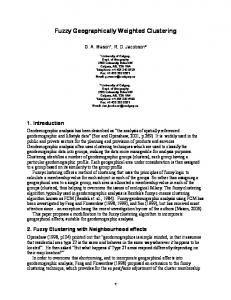
Fig. 1. Maps of tree locations for the three example plots: (a) regularity, (b) randomness, and (c) clustering. The circle is proportional to the tree DBH.
Table 1. Goodness-of-fit test for the improvement of the geographically weighted regression (GWR) models over the ordinary least-square (OLS) model for the 48 plots.
40
Spatial weighting GWR
Spatial-attribute weighting GWR
Plot
Fa
F
01 02 03 04 05 06 07 08 09 10 11 12 13 15 16 17 18 19 20 21 22 25 26 29 30 31 32 33 34 35 36 37 38 39 40 41 42 43 45 46 47 49 50 51 53 54 56 59
2.5223 2.0390 5.2687 6.1597 3.9897 2.4673 2.2733 2.3188 1.8045 1.9815 2.0855 1.6308 2.2761 1.7089 1.5265 2.7232 3.1648 4.6006 1.2741 1.9180 4.2975 2.9870 1.7848 3.7249 2.0904 2.0691 3.9460 3.4593 2.7529 1.0696 2.5141 5.3968 3.0901 2.0412 2.2591 4.3077 3.0153 5.7198 1.1837 2.3584 3.6691 2.3901 2.3224 3.8221 3.3976 1.8322 3.1504 4.8137
(a) 35 30
Y (m)
25 20 15 10 5 0 0
5
10
15
20
25
30
35
40
25
30
35
40
X (m)
40
(b)
35 30
Y (m)
25 20 15 10 5 0 0
5
10
15
20 X (m)
40
(c)
35 30
Y (m)
25 20 15 10 5
a
Pa 0.0017 0.0130