Our tool has a Java based interface and uses the statistical programming language R ... wizard. Keywords: software reliability, software testing, statistical models, R. 1 Introduction .... This options can be saved (or load) to (from) a .txt file. 6. Exit.
A New Statistical Software Reliability Tool M.A.A. Boon1 , E. Brandt2 , I. Corro Ramos1 , A. Di Bucchianico1 and R. Henzen2 1
Department of Mathematics, Eindhoven University of Technology, Eindhoven, The Netherlands 2
Refis System Reliability Engineering, Bilthoven, The Netherlands
Abstract We describe a new statistical tool for software reliability analyses that we are developing. Existing packages for statistical analysis of software reliability data do not make full use of state-of-the-art statistical methodology or do not conform to best practices in statistics. Our tool has a Java based interface and uses the statistical programming language R (see www.r-project.org) for the statistical computations. R is open-source free software maintained by a group of top-level statisticians and is rapidly becoming the standard programming language within the statistical community. The tool has a user-friendly interface which includes features like autodetection of datatype and a model selection wizard.
Keywords:
1
software reliability, software testing, statistical models, R.
Introduction
Successful testing processes require excellence in both software testing and management. In order to support well-founded decisions on issues like resource allocation and software release moments, quantitative procedures are indispensable. Since few testing processes have a deterministic course, statistics is very often an appropriate part of such quantitative procedures. Existing tools for software reliability analysis like Casre and Smerfs3 do not make full use of state-of-the-art statistical methodology or do not conform to best practices in statistics. Thus, these tools cannot fully support sound software reliability analyses. We decided to build a new tool that • uses well-documented state-of-the-art algorithms • is platform independent • encourages to apply best practices from statistics • can easily be extended to incorporate new models. In order to meet these requirements we decided to use Java for the interface and the statistical programming language R (see www.r-project.org) for the statistical computations. R is opensource free software maintained by a group of top-level statisticians and is rapidly becoming the standard programming language within the statistical community. In this paper we report on the status of our tool. Our tool is a joint project of the Laboratory for Quality Software (LaQuSo) of the Eindhoven University of Technology (www.laquso.com) and Refis 1
(www.refis.nl). The tool development is financially supported by a grant of the Dutch Innovation Platform. The rest of the paper is organized as follows. In Section 2 general guidelines of software reliability analysis are given. In Section 3 we present general and statistical features of the tool. We focus on describing the tool’s GUI thoroughly. A study to show how the tool works in practice is presented in Section 4. Finally, in Section 5 we summarize the work carried out and we point out to several important short-term objectives.
2
A note on reliability analysis
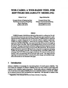
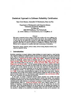
For general information on software reliability analysis we refer to Lyu (1996), Musa (2006) and Pham (2006). Like there exist coding standards for writing software, there also exist standards for performing statistical analyses. Basic steps in a statistical analysis of software reliability data should include (cf. Goel (1985)) 1. data collection (which data is relevant for the analysis) 2. trend tests (does the data indicate growth, otherwise analysis is useless) 3. model selection (pre-selection of models) 4. model estimation (calculate optimal parameters from data) 5. model validation (do models fit to data) 6. model interpretation (calculate quantities of interest from model parameters). We talk of ungrouped or exact data when the failures are reported individually and the data represents time between failures. However, it is possible to report faults in periods of time, in which case the data consists of the time intervals where the failures are reported and the number or faults found in each intervals. In this case we talk of grouped or interval data. Unfortunately, ungrouped data has received much more attention in the literature. Before trying to fit any reliability growth model, we should verify whether the data indicates reliability growth. This can be done using adequate plots or more formally with trend tests. Figure 1 clearly depicts the idea that software becomes more reliable as long as it is tested and errors have been repaired, so that more effort is required to find future errors. There are over 200 models based on different assumptions, assumptions which are often unclear or too unrealistic. Systematic approaches to use model assumptions and data requirements for initial model selection have not received much attention in the literature, Kharchenko et al. (2002) being an exception. Therefore, we have been developing a matrixbased procedure to support the choice of the models to work with. A simple version of this matrix can be found in Figure 2. Since we wish to select rather than rule out applicable models, we state all assumptions as negations of restrictions. To select models, one first has to select relevant assumptions and weights to incorporate the available information on the testing project at hand. If all requirements and selected assumptions of a model are satisfied, then the score for this model is 100%. In all other cases the score of the model is defined using the relative importance (weight) of the applicable characteristics of the model. Estimation of model parameters requires optimization. Since the parameters typically are of different order of magnitude, numerical problems like non-convergence or large flat areas 2
Figure 1: Reliability growth data. around the maximum cause practical problems (see Yin and Trivedi (1999)). In our tool we pay attention to convergence issues and apply algorithms that avoid the standard numerical problems. After parameter estimation has been completed, model verification must be determined. Graphical methods like the u-plot or TTT (Total Time on Test) plots (see Rigdon and Basu (2000) for details) or goodness-of-fit tests can be applied. Unluckily we find also problems here (derived to the fact that the assumptions of independent and identically distributed observations are normally broken by software reliability models). Therefore, standard goodness-of-fit tests, like the Kolmogorov test, cannot be used although this is often done. For diverse subclasses of models new goodness-of-fit tests are becoming available (see Bhattacharjee et al. (2004), Zhao and Wang (2005)). Finally, model interpretation makes possible to determine quantities like number of remaining errors and reliability of the system.
3
Software reliability tool
In this section we give a general overview of the GUI of our tool. Our tool is written in Java and we have made use of readily available components from Java Resource Bundles. The statistical computations are performed by calling R (high-quality free open source statistical software). The communication of Java with R uses JRI and JavaGD libraries developed by RoSuDa, the Computational Statistics group of the University of Augsburg. Initially, the GUI of our tool consists of four menu items as we can see in Figure 3. The multiple options 3
Figure 2: Assumption matrix. of all the menus are explained during this section. In the beginning only the Data and Help menus are enabled. To have access to the working environment we have to select the option Import from Data menu. We can distinguish two new windows that will remain visible all the time, one devoted to data and the other one to graphics. Figure 4 shows the data window. Three different tabs can be identified. The first one contains the imported data, the second one is allocated to the filtered data (in case we use this option) and the third one will show the data from the model analysis. Figure 1 shows the Graphical Output window where all the plots produced will be displayed. In the rest of this section we explain the tool menu options in detail, paying special attention to the Models and Analysis menus.
3.1
Data menu
1. Import Imports data files in .txt and .xls formats. After loading the data set the working environment is displayed. 2. Export Exports data files in .txt and .xls formats. 3. Filter Data This dialog (see Figure 5) allows to refine the data set and keep a subset of observations. The filtered data set can be also exported and imported. 4
Figure 3: Software reliability tool GUI.
Figure 4: Data window. 4. Transform Variable With this option we can create new variables applying basic operations to the variables of the data set. The available operations can be observed in Figure 6. 5. Preferences User preferences can be set using this option. Font type and size can be chosen for both program GUI and output (see Figure 7). The number of significant digits can be selected from one up to eight (by default set to three). We can also decide the colours 5
Figure 5: Filter Data dialog.
Figure 6: Transform Variable dialog. to be used in the plots. This options can be saved (or load) to (from) a .txt file. 6. Exit Closes the GUI and terminates the program execution.
3.2
Graphics menu
1. Create Scatter Plot With this option we can generate plots that will be loaded in the Graphical Output window. After clicking on this item, a window named Select Plot Variables pops-up (see Figure 8). We can select the variables we want to plot and assign them to the X or Y axes. We can choose as well the type of plot we desire to generate. The options are scatter plot, normal probability plot or TTT plot. Finally, the Draw Graph button will create the graph. In the lower part of the window we can set the display options of the plot like the main title, the labels of the axes or the format of the curves.
6
Figure 7: Preferences window.
Figure 8: Select Plot Variables window. 2. Copy Current Plot to Clipboard Copy the plot that is displayed in the Graphical Output window to the clipboard. Thus, the plot is cached and can be transferred between documents or applications, via copy and paste operations. 3. Export Current Plot Selecting this option, a save dialog appears to export the current plot to a graphic file. The formats supported are .eps, .jpg and .png. 4. Print Current Plot
7
With this option, a print dialog is displayed to print the current plot.
3.3
Analysis menu
1. Model Select Wizard Figure 9 shows the Model Select Wizard. In this dialog a list of common software reliability assumptions are enumerated. These assumptions are known from the literature and they are used in different software reliability models. The most relevant models are listed on the right-hand side of the dialog follow by a column called Score. Every assumption has a score associated to every model. After selecting the assumptions, the models receive points and they are sorted by relevance. The higher score a model has, the better the model will fit the assumptions.
Figure 9: Model Select Wizard dialog. 2. Data Type With the Select Data Type window (see Figure 10) we have the option to set the type of data of our data set. Time between failures or cumulative times, exact or interval data are the available options. In case of interval data we have to distinguish between counts per interval or cumulative counts. Options like different kind of errors (severity) or whether the last element of the data set is an observer error, are also possible. In case we do not know which kind of data we have, the option Try to Autodetect Data Type results of special interest. With this button the program estimates the type of data of our data file. Checking the number of columns (grouped or un-grouped) or the growth of the data (time between failures or cumulative times) we may find out what kind of data we are using. 3. Trend Tests The tool has the Laplace and the MIL-HDBK 189 trend tests already implemented and new tests will be added soon. The Trend Tests window is shown in Figure 11. Select
8
Figure 10: Select Data Type dialog.
Figure 11: Trend Tests window. the variable whose growth we want to test as well as the tests we would like to use. Also the confidence at which the test will be performed can be selected here. In the righthand side of the window we can observe the result of the tests we decided to perform. Graphical interpretation of the test is also displayed in the Graphical Output window. 4. Analyse Model The analysis window is shown in Figure 12. Before performing the analysis four steps must be follow. First, select the model(s) to fit the data. Then, set the confidence level used to calculate confidence intervals (by default set to 95%) and the significance level to perform hypothesis testing (by default set to 1%). Last, choose between the maximum-likelihood or least squares methods for parameter estimation. To perform the analysis click on Analyse Model button. Subsequently, the analysis output shows the 9
Figure 12: Analysis output. data type, the model choices, the parameter estimates and the result of the Kolmogorov goodness-of-fit test. The data window (see Figure 13) presents the the fitted values for the selected models. Finally, the graphical output (see Figure 14) shows the observed
Figure 13: Fitted values data.
10
values and the estimated models (by default represented by circles and a solid curve, respectively).
Figure 14: Fitted model plot. 5. Plot Fitted Models This option is enabled only after the analysis has been done and allows us to plot the observed values and the estimated models we selected for the analysis. 6. Export Output to Excel This option is also enabled only after the analysis has been performed and give us the possibility to export the output of the analysis to .xls format.
3.4
Help menu
1. Tool Help Help files of the tool. 2. SRE Help Glossary of terms and background on chosen algorithms. 3. About. . . Information about the developers, version of the tool, etc. . .
11
4
Case study
In this section, we show a demonstration of the tool using a data set by Joe (1989). The data set, reproduced in Table 1, consists of 207 observations corresponding to times between failures (ungrouped data). To load the data set in our tool click on Data menu and then
39 42 186 5 165 22 14 1 240 6 19 84 80 212 317
10 9 53 22 14 15 24 150 178 193 128 232 245 91 500
4 49 14 36 22 19 12 382 34 27 34 108 196 3 673
36 44 9 35 41 42 159 160 102 25 84 38 46 10 432
4 32 2 121 12 14 89 66 9 96 40 86 152 172 66
Joe I data set 5 4 91 49 3 78 1 30 10 1 34 170 23 33 48 32 138 95 49 62 11 41 210 16 118 29 21 18 206 9 26 62 146 59 48 25 26 30 30 17 177 349 274 82 7 22 80 239 102 9 228 220 21 173 371 40 168 66 66 128
1 205 129 21 2 30 2 239 25 320 58 3 208 48 49
25 5 4 4 35 37 114 13 111 78 31 39 78 126 332
1 129 4 23 89 66 37 4 5 39 114 63 3 90
4 103 35 9 99 9 46 85 31 13 39 152 83 149
30 224 5 13 69 16 17 85 51 13 88 63 6 30
Table 1: Time between failures. Import. An open dialog pops up (see Figure 15). We look for the data file that contains our data set (Joe I.xls) and then we click Open. We can distinguish three different windows in the GUI as we mentioned in the beginning of Section 3. In the left-hand side we can observe the data file while the graphical output window appears in the right-hand side. The middle of the screen is occupied by the Select Data Type dialog, already presented in Section 3.3 as part of the Data Type menu (see Figure 10). With this dialog we decide the kind of data we have. Therefore, select Time between errors and Ungrouped options. Note that in case of doubt we can try the option Try to Autodetect Data Type. The next step is to check whether the data presents any trend. Select the option Trend Tests from the Analysis menu and the Trend Tests window will be displayed (see Section 3.3, Trend Tests). Select the variable Cumulative Times follow by the trend tests we want to perform, in this case both Laplace and MIL-HDBK 189. Set the statistical confidence level (Alpha) for the analysis and then, click on Perform Test. The results of the tests are shown in Figure 11. On the Test Results area we can observe that both tests support the fact that there exists significant growth in reliability. In addition, the graphical output displays a graphical interpretation of the (statistical) test (in this case MIL-HDBK 189 test) as we can appreciate in Figure 16. Since the result of the trend test is positive, i.e., the data shows reliability growth, the next step is to perform analysis of the data applying software reliability models. An initial model inspection can be done with the option Model Select Wizard from the Analysis menu, as we described in Section 3.3 (see Figure 9). Choose the most appropriate assumptions to our case and select the model (or models) with the highest score. In this case, Goel-Okumoto seems to be a suitable model for our assumptions, as we can appreciate in Figure 17. Select Analyse Model from the Analysis 12
Figure 15: Browsing the data file.
Figure 16: MIL-HDBK 189 trend test graphical interpretation. menu and the analysis output window (see Figure 12) will be displayed. Select Goel-Okumoto model and set the confidence level used to calculate confidence intervals and the significance level to perform hypothesis testing. Choose between maximum likelihood or least squares parameter estimation methods and click on Analyse model. The result of the analysis is shown in Figure 18. The data window presents the fitted values for Goel-Okumoto model.
13
Figure 17: After selecting our assumptions, Goel-Okumoto model gets the highest score.
Figure 18: Model analysis. The graphical output shows the observed values (circles) and the estimated model (curve). A first inspection of this plot suggests that Goel-Okumoto is a reasonable model for our data. Formal result of the analysis (parameter estimates and goodness-of-fit test) is displayed in the analysis output window. As a consequence of our analysis we can conclude that there is no eveidence to reject the fact that our data can be described using Goel-Okumoto model.
14
5
Conclusions and future work
We have developed a new tool for statistical software reliability analyses. The interface is programmed in Java and therefore, it is platform independent. Our tool uses well-documented state-of-the-art statistical algorithms programmed in R and encourages to apply best practices from statistics. Furthermore, it has a user-friendly interface which includes features like model selection wizard and autodetection of datatype. The extension of the tool incorporating new models and features it is an ongoing challenge that stimulates us to continue working on this direction.
References M. Bhattacharjee, J. V. Deshpande, and U. V. Naik-Nimbalkar. Unconditional tests of goodness of fit for the intensity of time-truncated nonhomogeneous Poisson processes. Technometrics, 46(3):330–338, 2004. A.L. Goel. Software reliability models: Assumptions, limitations, and applicability. IEEE Trans. Soft. Eng., 11(12):1411–1423, 1985. H. Joe. Statistical inference for General-Order-Statistics and Nonhomogeneous-PoissonProcess software reliability models. IEEE Trans. Software Eng., 15(11):1485–1490, 1989. V.S. Kharchenko, O.M. Tarasyuk, V.V. Sklyar, and V.Yu. Dubnitsky. The method of software reliability growth models choice using assumptions matrix. In COMPSAC ’02: Proceedings of the 26th International Computer Software and Applications Conference on Prolonging Software Life: Development and Redevelopment, pages 541–546, Washington, DC, USA, 2002. IEEE Computer Society. M.R. Lyu, editor. Handbook of Software Reliability Engineering. McGraw-Hill and IEEE Computer Society, New York, 1996. J.D. Musa. Software Reliability Engineering: More Reliable Software Faster and Cheaper. Author House, Bloomington, USA, 2nd edition, 2006. M. Ohba. Software reliability analysis models. IBM J. Res. Develop., 28(4):428–443, 1984. H. Pham. System Software Reliability. Springer Series in Reliability Engineering. Springer, London, 2006. S.E. Rigdon and A.P. Basu. Statistical Methods for the Reliability of Repairable Systems. Wiley, 2000. M. Xie, Y.-S. Dai, and K.-L. Poh. Computing Systems Reliability. Models and Analysis. Kluwer, New York, 2004. L. Yin and K.S. Trivedi. Confidence interval estimation of NHPP-based software reliability models. In Proc. 10th Int. Symp. Software Reliability Engineering (ISSRE 1999), pages 6–11, 1999. J. Zhao and J. Wang. A new goodness-of-fit test based on the Laplace statistic for a large class of NHPP models. Comm. Statist. Simulation Comput., 34(3):725–736, 2005. 15