A new stratospheric and tropospheric NO2 retrieval algorithm for nadir ...

Open Access

Atmospheric Measurement Techniques

Atmos. Meas. Tech., 6, 2607–2626, 2013 www.atmos-meas-tech.net/6/2607/2013/ doi:10.5194/amt-6-2607-2013 © Author(s) 2013. CC Attribution 3.0 License.

A new stratospheric and tropospheric NO2 retrieval algorithm for nadir-viewing satellite instruments: applications to OMI E. J. Bucsela1 , N. A. Krotkov2 , E. A. Celarier2,3 , L. N. Lamsal2,3 , W. H. Swartz2,4 , P. K. Bhartia2 , K. F. Boersma5,6 , J. P. Veefkind5 , J. F. Gleason2 , and K. E. Pickering2 1 SRI

International, Menlo Park, CA 94025, USA for Atmospheres, NASA Goddard Space Flight Center, Greenbelt, MD 20771, USA 3 Universities Space Research Association, Columbia, MD 21044, USA 4 Applied Physics Laboratory, The Johns Hopkins University, Laurel, MD 20723, USA 5 Royal Netherlands Meteorological Institute, De Bilt, the Netherlands 6 Eindhoven University of Technology, Eindhoven, the Netherlands 2 Laboratory

Correspondence to: E. J. Bucsela ([email protected]) Received: 20 November 2012 – Published in Atmos. Meas. Tech. Discuss.: 7 February 2013 Revised: 12 July 2013 – Accepted: 1 August 2013 – Published: 15 October 2013

Abstract. We describe a new algorithm for the retrieval of nitrogen dioxide (NO2 ) vertical columns from nadir-viewing satellite instruments. This algorithm (SP2) is the basis for the Version 2.1 OMI This algorithm (SP2) is the basis for the Version 2.1 Ozone Monitoring Instrument (OMI) NO2 Standard Product and features a novel method for separating the stratospheric and tropospheric columns. NO2 Standard Product and features a novel method for separating the stratospheric and tropospheric columns. The approach estimates the stratospheric NO2 directly from satellite data without using stratospheric chemical transport models or assuming any global zonal wave pattern. Tropospheric NO2 columns are retrieved using air mass factors derived from high-resolution radiative transfer calculations and a monthly climatology of NO2 profile shapes. We also present details of how uncertainties in the retrieved columns are estimated. The sensitivity of the retrieval to assumptions made in the stratosphere– troposphere separation is discussed and shown to be small, in an absolute sense, for most regions. We compare daily and monthly mean global OMI NO2 retrievals using the SP2 algorithm with those of the original Version 1 Standard Product (SP1) and the Dutch DOMINO product. The SP2 retrievals yield significantly smaller summertime tropospheric columns than SP1, particularly in polluted regions, and are more consistent with validation studies. SP2 retrievals are also relatively free of modeling artifacts and negative tropospheric NO2 values. In a reanalysis of an INTEX-B valida-

tion study, we show that SP2 largely eliminates an ∼20 % discrepancy that existed between OMI and independent in situ springtime NO2 SP1 measurements.

1

Introduction

Nitrogen oxides are important atmospheric trace gases that have significant impacts on human health. The two principal nitrogen oxides, nitric oxide (NO) and nitrogen dioxide (NO2 ) (collectively NOx ), play key roles in atmospheric aerosol formation and tropospheric ozone chemistry (e.g., Finlayson-Pitts and Pitts, 1999; Seinfeld and Pandis, 1998). Major sources of tropospheric NOx include combustion, soil emissions, and lightning. In the lower troposphere, NO2 is a toxic gas and a precursor to tropospheric ozone through the reaction of NOx with volatile organic compounds (VOCs). In the stratosphere, NOx contributes to both production and loss cycles of ozone and may indicate long-term changes in tropospheric emissions of nitrous oxide (N2 O), an important greenhouse gas. Stratospheric NOx is produced mainly by the reaction of N2 O with O(1 D). NO2 has an easily observable spectral signature with strong spectral absorption lines in the visible, infrared, and near ultraviolet. In particular, its broad, highly structured absorption feature in the blue-violet range can be exploited for remote sensing (Platt and Perner, 1983; Platt, 1994).

Published by Copernicus Publications on behalf of the European Geosciences Union.

2608

E. J. Bucsela et al.: New NO2 retrieval algorithm for nadir-viewing satellite instruments

Early spectroscopic ground-based measurements of NO2 were described by Brewer et al. (1973), Noxon (1975), and Solomon and Garcia (1984). Global retrievals from satellite spectra became available beginning in the middle 1990s, including measurements by the Global Ozone Monitoring Experiment (GOME) instrument (1995–2003) (Burrows et al., 1999), continued by the Scanning Imaging Spectrometer for Atmospheric Cartography (SCIAMACHY) instrument (2002–2012) (Bovensmann et al., 1999), and currently by the Ozone Monitoring Instrument (OMI) (Levelt et al., 2006; Bucsela et al., 2006; Boersma et al., 2007, 2011) and GOME-2 (Callies et al., 2000; Valks and Loyola, 2008; Valks et al., 2011) instrument. Satellite and in situ measurements of tropospheric nitrogen oxides are used with chemical transport models (CTMs) to quantify sources and transport of NO2 pollution from power plants, automobiles, ships, and aircraft (e.g., Martin et al., 2003, 2006; Zhang et al., 2007; Beirle et al., 2004, 2011; Jaeglé et al., 2005; Frost et al., 2006; Boersma et al., 2008; Lin et al., 2010; Russell et al., 2010). Instruments on satellite platforms are particularly valuable, since they can obtain NO2 measurements over large geographical regions. Top-down NO2 measurements are helpful in constraining emissions for global- and regional-scale atmospheric models (Martin et al., 2003; Choi et al., 2008; Lamsal et al., 2010). Multiyear, consistent time-series measurements allow the study of interannual variability and long-term trends (Richter et al., 2005), which have been used to assess the effectiveness of emission control regulations and the effects of economic trends on industrial activity (Frost et al., 2006; Kim et al., 2006; Castellanos and Boersma, 2012). NOx produced by lightning (LNOx ) contributes an additional 10– 15 % to total NOx production in the troposphere (Schumann and Huntrieser, 2007), and LNOx measurements are helpful in estimating the global NOx budget (Tie et al., 2002; Martin et al., 2007). In unpolluted areas, the stratospheric NO2 can exceed 90 % of the total NO2 column (Martin et al., 2002a). The partitioning of NOx and NOy in the stratosphere is sensitive to photochemical conditions; thus, NO2 has a strong diurnal dependence that varies as a function of latitude and season (Dirksen et al., 2011). Although NO2 in the stratosphere is more zonally symmetric than in the troposphere, there is still spatial structure that is important for understanding the morphology of stratospheric NO2 itself, while complicating the retrieval of tropospheric NO2 from satellite-derived slant columns. The accuracy of the inferred tropospheric contribution critically depends on the characterization and separation of stratospheric NO2 . The procedure used to determine the two components of the NO2 vertical column will be referred to as the stratosphere–troposphere separation (STS) algorithm. Determining the relative amounts of stratospheric and tropospheric NO2 from a given absorption spectrum is inherently difficult. Although the shape of the NO2 absorption Atmos. Meas. Tech., 6, 2607–2626, 2013

cross section varies with altitude (due to temperature), cross sections at different temperatures are not orthogonal. Therefore, the stratospheric and tropospheric NO2 amounts cannot be independently determined from the spectral fit. Instead, most STS algorithms rely on spatial information from multiple slant columns measured over a wide geographic area. All such algorithms are prone to errors associated with the a priori information assumed about the stratospheric vertical column. The reference-sector (RS) method, discussed by Richter and Burrows (2002) and Boersma et al. (2004), assumes zonal invariance. The stratospheric vertical column at any latitude is set equal to the measured total column at the same latitude in the central Pacific Ocean. Because the central Pacific contains small background amounts of tropospheric NO2 , the RS method can slightly overestimate the stratospheric fraction of the column. Martin et al. (2002a) corrected this by using model estimates of Pacific tropospheric NO2 . More importantly, the real stratospheric NO2 varies with longitude, leading to potential inaccuracies in both the stratospheric and derived tropospheric vertical column. Other methods, such as the image processing technique (IPT) of Leue et al. (2001) and Velders et al. (2001), and the wave-2 stratospheric model of Bucsela et al. (2006), allow for some longitudinal variation in stratospheric NO2 . However, like the RS method, the IPT and wave-2 algorithms required relatively simplistic assumptions about which regions to use in constructing the global NO2 stratospheric field. The wave-2 model, in particular, can introduce stratospheric artifacts, especially at high latitudes (Dirksen et al., 2011). Some approaches have tried to capture more realistic structure in the stratospheric NO2 field by using CTMs to estimate the spatial variation in stratospheric NO2 . In the Dutch OMI NO2 (DOMINO) product (Boersma et al., 2011; Dirksen et al., 2011), OMI NO2 measurements are assimilated in a CTM model. CTM-based algorithms require daily model runs and relatively complex assimilation schemes. As will be shown, CTM-based algorithms can also introduce occasional modeling artifacts. If independent stratospheric measurements are available, a more observation-based approach can be used. Beirle et al. (2010) and Hilboll et al. (2013) have described methods for combining nadir measurements from OMI or SCIAMACHY with limb measurements of stratospheric NO2 from SCIAMACHY. Because the limb measurements are sparsely sampled, these approaches require significant spatial interpolation to obtain a continuous stratospheric field. In this paper, we describe a new algorithm for the retrieval of NO2 vertical columns using only nadir-viewing satellite slant-column measurements, simple tropospheric climatologies, masking and interpolation. The algorithm is now used to produce NASA’s Version 2 OMI NO2 (OMNO2) Standard Product (SP2), and could be employed for other satellite measurements. For OMI data, SP2 is a significant improvement over the original SP1, which was based on the wave-2 STS algorithm. SP2 continues the philosophy of minimizing www.atmos-meas-tech.net/6/2607/2013/


2609

Table 1. Comparison of SP1 and SP2. Algorithm component Stripe correction

SP1 (Released 2006)

SP2 (Released 2011)

Based on data from 60◦ S–60◦ N of

Based on data from 30◦ S–5◦ N of 5 orbits.

15 orbits. Stratosphere–troposphere separation

Air Mass Factor (AMF)

NO2 profile shape

Temperature profile Scattering weights Terrain albedo Tropopause pressure Cloud pressure/fraction

Stratospheric NO2 field based on a global analysis, assuming a zonal wave-2 structure.

In regions of tropospheric pollution, stratospheric column is inferred using a local analysis of the stratospheric field.

GEOS-Chem annual mean tropospheric NO2 profiles for the year 1997 coupled with a single stratospheric profile. NMC monthly profile climatology. Tabulated results from TOMRAD simulation. GOME(-1)-based monthly climatology. Fixed tropopause pressure. O2 -O2 cloud algorithm.

Monthly mean NO2 profile shapes derived from GMI CTM multiannual (2005–2007) simulation.

the use of model information in retrievals, but includes a number of features not present in SP1. The SP2 stratospheric slant column is estimated from the total slant column using an a priori monthly tropospheric NO2 model climatology, but only where tropospheric contamination of the observed NO2 column is below a threshold. The threshold is set by an upper limit on the amount that tropospheric NO2 absorption may contaminate the observed stratospheric vertical column. The SP2 algorithm also features improved air mass factors based on new radiative transfer calculations and terrain reflectivities and uses monthly, rather than annual, mean NO2 profile shapes. Cloud properties are obtained from the OMI OMCLDO2 data product, which has recently been updated to include better wavelength calibration, look-up tables using sun-normalized radiances, and cloud pressures clipped at the surface pressures (Maarten Sneep, private communication). The purpose of this paper is twofold: (1) to introduce the new STS algorithm and (2) to discuss the additional, more incremental changes that distinguish SP2 from SP1. We describe the algorithm in Sect. 2 and list the differences between the old and new retrieval approaches. We present error analysis in Sect. 3 and discuss additional considerations and comparisons with other datasets in Sect. 4. Although a thorough treatment of validations comparing the new algorithm with independent datasets is beyond the scope of this paper, a validation example is included in Sect. 4. Numerous additional validation studies will be presented separately by Lamsal et al. (2013). Section 5 contains a summary and conclusions.

www.atmos-meas-tech.net/6/2607/2013/

2

GEOS-5 monthly profile climatology. Same, but with greater number of node points to reduce interpolation errors. OMI-based monthly climatology. GEOS-5 monthly tropopause pressure. Updated O2 -O2 cloud algorithm.

Algorithm description

The architecture of the algorithm is summarized in the flow diagram in Fig. 1. Spectral data are fitted to obtain raw NO2 slant columns, S 0 (Sect. 2.1), and are corrected for instrumental artifacts (also referred to as striping; see Sect. 2.3) to yield the de-striped slant columns, S. The data are analyzed to separate stratospheric and tropospheric NO2 partial vertical columns, Vstrat and Vtrop , and to obtain total column amounts, Vtotal (Sect. 2.4). The stratospheric and tropospheric air mass factors, Astrat and Atrop (Sect. 2.2), used in the calculations are based on a priori information from radiative transfer (RT) and CTM models. The RT calculations used to process the OMI data in this study were carried out using TOMRAD (Davé, 1965). Some details in the SP2 algorithm are similar to the approach used in SP1, but there are many important changes. The similarities and differences are summarized in Table 1, and details of the SP2 algorithm are presented in Sects. 2.1–2.4. 2.1

OMI spectral fitting

The NO2 slant columns used in this study were extracted from OMI spectra. The OMI instrument is a UV-VIS hyperspectral, push-broom, nadir-viewing satellite spectrometer (Levelt et al., 2006) on the NASA EOS Aura satellite (Schoeberl et al., 2006), launched in July 2004. Aura has an Equator crossing time of 13:30 LST and an orbital period of 99 min so that OMI views the entire sunlit portion of the Earth in ∼14.5 orbits. On each orbit, OMI makes simultaneous measurements in a swath width of ∼2600 km, divided into 60 fields of view (FOVs) or pixels. One swath is measured every two seconds, for approximately 1650 swaths from southern Atmos. Meas. Tech., 6, 2607–2626, 2013

2610

E. J. Bucsela et al.: New NO2 retrieval algorithm for nadir-viewing satellite instruments some extent using the “de-striping” procedure described in Sect. 2.3. A more severe effect is the “row anomaly” (RA), which was first noticed in the data in June 2007 and is likely caused by an obstruction in part of OMI’s aperture. The extent of the RA has increased since 2007 and currently affects approximately half of the FOVs. Current RA information is available at http://www.knmi.nl/omi/research/product/ rowanomaly-background.php. Users of OMI data are discouraged from using FOVs flagged as RA-affected.

Fig. 1. Flow diagram of retrieval algorithm for stratospheric and tropospheric NO2 columns. S, V , A, and SW represent slant-column density, vertical-column density, air mass factor, and scattering weight (m), respectively. The section outlined in blue is OMIspecific. TOMRAD is a forward vector radiative transfer model (Davé, 1965).

to northern terminator on the sunlit side of the earth. Swaths in adjacent orbits are nearly contiguous at the Equator and overlap elsewhere. LST differences from the west to east sides of a swath range from approximately 1.5 h at the Equator to several hours at mid- to high latitudes. The NO2 slant columns are estimated by spectral fitting of OMI earthshine radiances. The fitting algorithm uses the Differential Optical Absorption Spectroscopy (DOAS) method (Platt and Stutz, 2006), applied in the spectral range of 405 nm to 465 nm (Boersma et al., 2002; Bucsela et al., 2006). The earthshine radiances are normalized by a reference OMI-measured solar irradiance spectrum [R(λ) = I (λ)/F (λ)]. The use of a static measured solar reference spectrum reduced much of the calibration-induced striping that was discovered soon after OMI operations began (Dobber et al., 2008). (The removal of residual striping is described in Sect. 2.3). The normalized spectra, R(λ), are fitted to laboratory-measured trace gas absorption spectra at a fixed stratospheric temperature (T0 = 220 K), a reference ring spectrum (Chance and Spurr, 1997), and a polynomial function that models the spectrally slowly varying scattering by clouds and aerosols and reflection by the Earth’s surface. In the current version, the only trace gas absorption spectra considered are those of NO2 (Vandaele et al., 1998), O3 (Bass and Johnsten, 1975), and H2 O (Harder and Brault, 1997). The temperature dependence of the NO2 cross section is accounted for later in the algorithm. The trace gas absorption spectra used were produced by convolving highresolution, laboratory-measured absorption spectra with the measured OMI slit function, measured pre-launch by Dirksen et al. (2006). The result of the spectral fit is the raw slantcolumn density for each OMI pixel. The calibrations of the 60 cross-track FOVs have relative biases that are observed to be persistent on time scales of several orbits to several days. As a result, the retrieved NO2 slant columns show a pattern of stripes running along each orbital track. This instrumental artifact can be corrected to Atmos. Meas. Tech., 6, 2607–2626, 2013

2.2

Air mass factors

In DOAS retrievals, the air mass factor, A, is the ratio of a slant column, S, to the vertical column, V , we want to retrieve. We write this relationship generically as A = S/V . The air mass factor is assumed to be wavelength-independent across the slant-column fitting window. In a given partial atmospheric region (stratosphere or troposphere), the air mass factor is computed as the ratio of the sum over layers of the slant sub-columns Si to the sum of vertical sub-columns Vi : A=

6i Si S = , V 6i Vi

(1)

where i is the layer index. The summation combines all layers in the appropriate partial atmospheric column. Temperature is assumed to be constant within a layer. Slant and vertical sub-columns can be represented as integrals over all pressures p within layer i: Z (2) Si = κ dp · ζ (p) · m(p) · α(p) i

and Z dp · ζ (p).

Vi = κ

(3)

i

Here, m(p) is the atmospheric scattering weight (also referred to as the “box” or “layer” air mass factor), α(p) is a temperature-correction factor for the NO2 absorption cross section, ζ (p) is the a priori NO2 mixing ratio, and κ is a constant equal to the reciprocal of the weight of an air molecule. The formulation in Eqs. (2) and (3) implicitly decouples atmospheric scattering and NO2 absorption, as described by Palmer et al. (2001), so that the m(p) are independent of NO2 amount. The temperature factor α(p) is needed to correct for the fixed-temperature NO2 cross section (T0 = 220 K) used in the slant-column fitting and can be written as a function of the local temperature T (p) as α(p) = 1 − 0.003 · [T (p) − T0 ].

(4)

The coefficient 0.003 (units K−1 ) was obtained empirically by fitting synthetic radiance spectra with NO2 cross sections measured at several temperatures. This coefficient is www.atmos-meas-tech.net/6/2607/2013/

E. J. Bucsela et al.: New NO2 retrieval algorithm for nadir-viewing satellite instruments in line with temperature correction coefficients proposed in Boersma et al. (2002, 2004). For partly cloudy scenes, we use an independent-pixel approximation for the air mass factor (e.g., Martin et al., 2002a) and express scattering weights as the weighted sum of cloudy and clear components, m(p)cloudy and m(p)clear , respectively: m(p) = w · m(p)cloudy + (1 − w) · m(p)clear .

(5)

Here the weighting factor, w, denotes cloud/aerosol radiance fraction (CRF), the fraction of the measured radiation that comes from clouds and aerosols. In the SP1 and SP2 algorithms, aerosols are not distinguished from clouds, since weakly absorbing aerosols can have similar effects on the air mass factor in some circumstances (Boersma et al., 2011). The effect of stratospheric aerosols is also not explicitly considered in the algorithm. The value of w is generally larger than the O2 -O2 geometrical cloud fraction at 470 nm since the clouds are assumed to be optically thick with an effective Lambertian albedo of 0.8 (Stammes et al., 2008). The cloudy and clear scattering weights for a given observation depend on parameters including viewing geometry, surface (terrain or cloud) pressure, and surface reflectivity. Scattering weights are computed and stored a priori in sixdimensional look-up tables (LUT) generated from a radiative transfer model. For clear-sky scattering weights, the six LUT parameters are solar zenith angle (SZA), viewing zenith angle (VZA), relative azimuth angle (RAA), terrain reflectivity (Rt ), terrain pressure (Pt ), and atmospheric pressure level, (p). For cloudy scattering weights, we treat clouds as opaque Lambertian surfaces and replace the terrain reflectivity and terrain pressure with cloud reflectivity (Rc = 0.8) and cloud optical centroid pressure (Pc ), respectively. The latter is estimated with the OMI O2 -O2 cloud algorithm (Acarreta et al., 2004; Sneep et al., 2008; M. Sneep et al., private communication, 2012). The SP2 scattering weights are computed from parameter sets that have been improved relative to SP1. In particular, the terrain reflectivities, which were derived from GOME (Koelemeijer et al., 2003) in SP1, are now based on OMI measurements (Kleipool et al., 2008). Terrain pressures are obtained as described by Boersma at al. (2011) from a 3 km digital elevation model provided with the Aura data. The reflectivities and other parameters are no longer assumed to vary linearly between tabulated values, as was the case in SP1, and are now interpolated using Lagrange polynomials. The resolution in the six-dimensional parameter space has also been increased. In the new algorithm, the number of nodal points in SZA, VZA, RAA, Rt , Pt , and p are 9, 6, 5, 8, 6, and 35, respectively. These improvements reduce interpolation errors noted in SP1 (Dirksen et al., 2011) by up to 15 %. The a priori NO2 mixing ratio profiles for the air mass factor calculations in SP2 are obtained 4 from the Global www.atmos-meas-tech.net/6/2607/2013/

2611

Modeling Initiative (GMI) CTM (Duncan et al., 2007; Strahan et al., 2007). The model simulates the stratosphere and troposphere and includes emissions, aerosol microphysics, chemistry, deposition, radiation, advection, and other important chemical and physical processes, such as lightning NOx production (Duncan et al., 2007). The GMI chemical mechanism combines the stratospheric mechanism described by Douglass et al. (2004) with a detailed tropospheric O3 -NOx -hydrocarbon chemistry originating from the Harvard GEOS-Chem model (Bey et al., 2001) and is driven by GEOS-5 meteorological fields at the resolution of 2◦ latitude × 2.5◦ longitude (Rienecker et al., 2008). The vertical extent of the model is from the surface to 0.01 hPa, with 72 levels and a vertical resolution ranging from ∼150 m in the boundary layer to ∼1 km in the free troposphere and lower stratosphere. The tropopause pressure is defined in the GEOS-5 reanalysis driving the CTM using a combination of Ertel’s potential vorticity (EPV) and potential temperature. The tropopause pressure is taken as the higher of the EPV = 3.6 × 10−6 K kg−1 m2 s−1 and 385 K theta surfaces. For the NO2 SP2 algorithm, the use of alternative tropopause definitions (e.g., a chemical tropopause) was found to have little effect on the retrieval, since the differences in pressure were generally small and occured in regions where NO2 concentrations are low. Model outputs were sampled at the LST of OMI overpass, and monthly mean profiles were derived using four years (2004–2007) of simulation. In contrast, SP1 used annual mean tropospheric profiles for 1997 from a GEOSChem simulation (Bey et al., 2001; Martin et al., 2002b), with only a single profile used for the stratosphere (Bucsela et al., 2006). Unlike the stratospheric air mass factor, which depends mainly on the viewing geometry, the air mass factor in the troposphere is particularly sensitive to the NO2 profile shape. Model profile shapes vary by geographic region and exhibit daily variability as well, as validated by in situ measurements (e.g., Boersma et al., 2008; Bucsela et al., 2008). Our sensitivity studies indicated that monthly mean profiles captured the seasonal variation sufficiently well so that daily profiles were not included in the SP2 algorithm; however, use of 30-day running mean NO2 profile shapes is being considered for a future version of the algorithm. 2.3

De-striped slant columns

As described in Sect. 2.1, an instrumental artifact introduces a bias in the retrieved OMI NO2 slant columns, resulting in the appearance of orbital “stripes” when the data are mapped. The de-striping algorithm computes the mean cross-track biases using raw NO2 slant columns and stratospheric air mass factors from five consecutive orbits over clean regions (30◦ S to 5◦ N). This approach relies on identifying and estimating cross-track bias in slant columns from cross-track variation in the stratospheric air mass factors. An initial estimate of the bias δi for each cross-track position i is computed Atmos. Meas. Tech., 6, 2607–2626, 2013

2612


1 Fig. 2. Maps of 21 March 2005 OMI NO2 data showing STS algorithm steps. (a) Slant columns. (b) Vinit . (c) Vinit minus a priori troposphere. 2 Figure 2: Maps of 21 March 2005 OMI NO2 data showing STS algorithm steps. (a) Slant o (d) Same as (c), but masked for pollution (white areas correspond to a masking threshold of 0.3 × 1015 cm−2 ). (e) Gridded, Vstrat with masked 3 columns. (b)removed. Vinit. (c) priori (d) Sameonto as (c), for (h) Tropospheric areas interpolated. (f) Hot spots (g)VStratosphere finaltroposphere. smooth, re-interpolated OMIbut pixelmasked coordinates. init minus aafter field. 15 –2

4

pollution (white areas correspond to a masking threshold of 0.3 ·10

cm ). (e) Gridded,

5 Vostrat with masked areas interpolated. (f) Hot-spots removed. (g) Stratosphere after final from the mean slant column ‹ S 0 ›i and stratospheric air mass fected by the RA) do not affect the average. The resulting 6 smooth, re-interpolated onto OMI pixel coordinates. (h) Tropospheric field. factor ‹ Astrat ›i for that cross-track position and the avercross-track bias for a given OMI orbit is a set of 60 correc7 age slant column ‹‹ S 0 ›i › and average stratospheric air mass tion constants. At each pixel in the orbit, the corresponding factor ‹‹ Astrat ›i › over the entire swath from 30◦ S to 5◦ N. bias is subtracted from the measured slant column S 0 to give The computation of the entire swath averages excludes all a corrected (“de-striped”) slant column S. scan positions that have extreme values of ‹ S 0 ›i /‹ Astrat ›i 2.4 Stratosphere–troposphere separation (STS) (> 1017 cm−2 ) and those known, a priori, to be affected by the row anomaly. The initial bias estimate is The STS scheme described in this study takes advantage of 0 0 the fact that, over most of the Earth, the NO 412 absorption conδi = ‹ S ›i − [‹ Astrat ›i · ‹‹ S ›i ›/‹‹ Astrat ›i ›]. (6) tributing to the slant-column measurements is almost entirely The final value of the cross-track bias is recomputed from stratospheric. Therefore, a simple and reasonable initial estiEq. (6) by applying an additional screening criterion in the mate of the stratospheric vertical column is the ratio of the calculation of ‹‹ S 0 ›i › and ‹‹ Astrat ›i ›. The cross-track scan de-striped measured slant column to the (nearly geometric) positions whose δi values lie outside a ±2σ interval are exstratospheric air mass factor: cluded to ensure that very high or low values of the bias in any of the cross-track scan positions (including those afVinit = S/Astrat . (7)

Atmos. Meas. Tech., 6, 2607–2626, 2013


E. J. Bucsela et al.: New NO2 retrieval algorithm for nadir-viewing satellite instruments In areas with relatively little tropospheric NO2 , we obtain the value of the stratospheric vertical column by subtracting a fixed model estimate of the (small) tropospheric column from Vinit and applying spatial smoothing to the resultant geographic field. Where there is substantial tropospheric NO2 pollution, the stratosphere is estimated by spatial interpolation from the surrounding clean regions. The tropospheric vertical column is then computed as the difference between S and the stratospheric slant column, divided by a tropospheric air mass factor. Figure 2 illustrates the steps of the STS algorithm for one day of data, beginning with the spectrally fitted slant columns (Fig. 2a) and initial vertical columns Vinit (Fig. 2b). The following seven steps summarize subsequent computations. 1. Subtract an a priori troposphere from Vinit to get initial stratospheric vertical column. 2. Mask the field wherever tropospheric contamination exceeds a threshold. 3. Bin this initial stratospheric vertical-column estimate onto a geographic grid. 4. Interpolate the binned vertical columns over masked areas. 5. Identify and eliminate “hot spots” in the stratospheric field. 6. Smooth and interpolate to pixel-center coordinates to give the final Vstrat at each FOV. 7. Subtract the stratospheric contribution to get the tropospheric vertical column. For steps 1 and 2, we first compute an a priori tropospheric slant column, Strop , at each satellite pixel: Strop = Vtrop_a_priori · Atrop ,

(8)

where Vtrop_a_priori is a geographically gridded (2◦ latitude × 2.5◦ longitude), monthly mean model of NO2 climatology of tropospheric vertical columns, and Atrop is the tropospheric air mass factor. The NO2 climatology used in computing Vtrop_a_priori is the same as that used in the calculation of Atrop . o (Fig. 2c) The initial estimate of the stratospheric field Vstrat is computed as o Vstrat = (S − Strop )/Astrat .

(9)

o for all pixels in which the troThe algorithm then masks Vstrat pospheric contamination of the NO2 column is large. Masked pixels, shown as white areas in Fig. 2d, are eliminated from the stratospheric field calculation. The masking threshold is chosen to exclude pixels where Vinit would exceed the actual


2613

stratospheric vertical column by more than a value ε. We require (Strop /Astrat ) < ε.

(10)

In the current algorithm, we chose an absolute threshold of ε = 0.3 × 1015 cm−2 to limit the stratospheric verticalcolumn uncertainty introduced by the a priori troposphere to a value of 0.2 × 1015 cm−2 or less. This uncertainty is consistent with previous estimates of uncertainty in the stratospheric NO2 column (see Sect. 3.2) and is comparable to pixel noise associated with the slant-column uncertainty (see Sect. 3). Using this masking scheme allows polluted pixels to remain unmasked where the lower troposphere is obscured by clouds. These unmasked pixels provide a more robust stratospheric retrieval in polluted areas than would be possible if all polluted regions were automatically masked. Leue et al. (2001) similarly made use of cloudy pixels to construct a stratospheric field relatively free of tropospheric contamination. Conversely, in regions where amounts of tropospheric NO2 are relatively small (∼0.5 × 1015 cm−2 ), tropospheric NO2 can still contaminate the measurements if skies are clear and surface reflectivities are high. Examples are the Sahara and southern Arabian Peninsula, which require more masking than similarly unpolluted ocean regions (see Fig. 2d). We have chosen an absolute, rather than relative, threshold to assess tropospheric contamination of the observed column, since using a relative threshold leads to unnecessary masking of areas where the magnitude of small stratospheric columns begins to approach the absolute measurement uncertainty. Globally, the fraction of pixels masked is approximately constant throughout the year and ranges from about 10 % in the Southern Hemisphere to nearly 35 % in the Northern Hemisphere. Steps 3–6 are performed with the stratospheric field data binned on a uniform 1◦ × 1◦ geographic grid. A separate global stratospheric field is constructed for each orbit by forming weighted averages of the data in each 1◦ × 1◦ bin and including data from the adjacent ± 7 orbits. Largest weights are assigned to data from the “target” orbit, so that adjacent orbits are essentially used only when data from the target orbit are unavailable. The weighting scheme minimizes the effects of mixing data from different local times in overlapping orbits with the data from the target orbit. Any unfilled bins in this vertical-column field are then interpolated using a 2-D averaging function in the form of a rectangular window of dimensions δLon in longitude and δLat degrees in latitude. At middle latitudes, we use a window of δLon ∼30◦ and δLat ∼20◦ , but we modify these values at low and high latitudes. In particular, the longitude dimension near the Equator is increased to 360 degrees to reduce synopticscale contamination of the stratospheric field by NO2 enhancements due to tropical lightning. Martin et al. (2007) have discussed the existence of longitudinally broad tropospheric LNO2 enhancements in the tropics between South America and Africa. The binned, interpolated field is shown Atmos. Meas. Tech., 6, 2607–2626, 2013

2614


in the grid-cell map of Fig. 2e. Note the scattered grid cells containing unmasked data within the smooth, interpolated (i.e., masked) field of Eastern Europe. These grid cells contain information responsible for the stratosphere’s structure in regions that otherwise may look to be uniformly masked in the orbital map of Fig. 2d. To further reduce contamination of the stratosphere by tropospheric NO2 not accounted for in the climatology, we use statistical criteria to identify and mask tropospheric hot spots (step 5). These may include unknown anthropogenic sources or intense, localized soil- and lightning-related emissions. For hot-spot removal, we employ a smaller averaging window of δLon ∼15◦ and δLat ∼10◦ . The Vstrat value in the bin at the center of the window is masked and replaced by the mean if its Vstrat exceeds the mean by more than 1.5 standard deviations. A comparison of Fig. 2e and f shows the result of the hot-spot removal. Note the removal of small areas of locally enhanced NO2 in Western Canada, the eastern Gulf of Mexico, and in various locations throughout Asia. Finally, the stratospheric vertical columns are smoothed using a small window of δLon ∼5◦ and δLat ∼3◦ and interpolated from the 1◦ × 1◦ grid back to the pixel-center coordinates. The smoothing step effectively degrades the spatial scale of resolvable stratospheric features to approximately 300 km so that any smaller-scale features in the Vinit field will be interpreted as tropospheric. The NO2 tropospheric column at each pixel is the difference between the total and the stratospheric columns, computed as follows: Vtrop = (S − Vstrat · Astrat )/Atrop ,

(11)

where S is the de-striped total measured slant column (Sect. 2.3) and Astrat and Atrop are the air mass factors (derived from a priori and cloud information as described in Sect. 2.2). Tropospheric values are generally positive, as seen in Fig. 2h, but local negative values may occur at any pixel where the binning, interpolation, and/or smoothing in the STS algorithm results in a Vstrat value larger than Vinit . The total column is the sum of the tropospheric and stratospheric columns: Vtotal = Vstrat + Vtrop .

(12)

Note that Vtotal is generally larger than Vinit , since Atrop is typically smaller than Astrat , especially where tropospheric NO2 is concentrated in the boundary layer and/or hidden by clouds. 3

Error estimates

The uncertainties in the total column amounts result from uncertainties in (1) the fitted NO2 slant columns, (2) the stratospheric and tropospheric air mass factors, and (3) the algorithm used to separate the stratosphere and troposphere Atmos. Meas. Tech., 6, 2607–2626, 2013

(STS). Descriptions of these errors in the context of OMI NO2 retrievals may be found in Boersma et al. (2004, 2011) and Wenig et al. (2008). The uncertainties in the slantcolumn amounts have been described previously (Boersma et al., 2004, 2011) and will not be discussed in detail here. For data collected during the first two to three years of the mission, the rms fitting error in the OMI NO2 slant column had a median value of approximately 1015 cm−2 , which is on the order of 10 % of the total slant column for polluted regions. For swath positions affected by the row anomaly (see Sect. 2.1), we calculate NO2 values but do not estimate uncertainties. We treat the S, A, and STS errors as statistically independent and discuss the latter two in Sects. 3.1 and 3.2. The combined errors for the vertical-column retrievals are given in Sect. 3.3. 3.1

Errors in air mass factors

The air mass factor (Astrat or Atrop ) is computed as shown in Eqs. (1–5). A general expression for the air-mass-factor uncertainty, σA , can be written as a sum of variances: (σA )2 = (σAm )2 + (σACTM )2 ,

(13)

where σAm is the net air-mass-factor error associated with the scattering weights, m, and σACTM is the net air-mass-factor error associated with the CTM used for the NO2 profile shape. The parameters that most affect the scattering weights are the terrain reflectivity, R, the cloud radiance fraction, w (w also implicitly accounts for aerosols; Boersma et al., 2011), and the effective cloud pressure (also referred to as optical centroid pressure), Pc . The parameters relating to the CTM are the NO2 sub-column profile, Vi , and temperature profile, Ti . In general, the uncertainties in these quantities are not independent; e.g., an overestimation of R can lead to an underestimation of w, and the derived cloud pressure Pc can also be related to w in cloud retrieval algorithms (Sneep et al., 2008). Likewise, the temperature profile Ti affects the model’s prediction of NO2 mixing ratios, ζ (p). Uncertainties in the viewing geometry and terrain pressure are neglected in this error formulation, although errors in the latter can affect integrated profile amounts, particularly over mountainous terrain (Schaub et al., 2007; Boersma et al., 2008; Hains et al., 2010; Russell et al., 2011). In spite of these interdependencies, we assume, for computational convenience, that these parameters can be decoupled as follows: (σAm )2 = (σAR )2 + (σAw )2 + (σAPc )2

(14)

and ζ

(σACTM )2 = (σA )2 + (σAT )2 ,

(15)

where σAR , σAw , and σAPc are the air-mass-factor errors due to errors in terrain reflectivity, R, cloud radiance fraction, w, www.atmos-meas-tech.net/6/2607/2013/

E. J. Bucsela et al.: New NO2 retrieval algorithm for nadir-viewing satellite instruments ζ

and cloud pressure, Pc , respectively. We also assume σA and σAT are the respective air-mass-factor errors due to errors in the model NO2 mixing-ratio profile, ζi , and temperature profile, Ti . We compute the terms on the right-hand sides of Eqs. (14) and (15) from Eqs. (1–5) and from a priori estimates of the uncertainties σR , σw , σPc , σζ , and σT in terrain reflectivity, cloud-radiance fraction, cloud pressure, NO2 profile, and temperature profile, respectively, and the sensitivities of A to each of these parameters. Using Eqs. (1–5), we can write β simplified expressions for the variances (σA )2 in the five parameters β = R, w, Pc , ζ , or T . If the atmosphere is divided into N vertical layers (i = 1, . . . N), we define an N-element Jacobian column vector Jβ and its (row) transpose JTβ . Each element (Jβ )i is the derivative of A (Eq. 1) with respect to parameter β in layer i. With these definitions, the five variances can be written in compact matrix notation, with the corresponding explicit expressions for the Jacobian elements as follows: 2 (σAR )2 = JT R (U · σR ) JR , Z (1 − w) κ · dp · (∂mclear /∂R ) · α · ζ, where (JR )i = V

(16)

i

(σAw )2

2 = JT w (U · σw )Jw ,

where (Jw )i = (σAPc )2

κ · V

Z

dp · (mcloudy − mclear ) · α · ζ,

(17)

i T 2 = JPc (U · σPc )JPc ,

where (JPc )i =

κ · V

Combining Eqs. (13–20), we summarize the net variance in the air mass factor as T 2 2 (σA )2 = JT R (U · σR )JR + Jw (U · σw )Jw + 2 JT Pc (U · σPc )JPc

dp · (∂m/∂Pc ) · α · ζ,

(18)

i ζ

(σA )2 = JT ζ Sζ Jζ , Z κ where (Jζ )i = · dp · (m · α − A), V

(19)

i

and (σAT )2 = JT T ST JT , Z −0.003 κ · dp · m · ζ. where (JT )i = V

(20)

i

In Eqs. (16–20), U is defined as an N × N-unit matrix (matrix of all elements equal to one). Sζ and ST are the N × N element covariance matrices for the a priori model NO2 mixing-ratio and temperature profiles, respectively. In general, for parameter β, the (i, j ) element of the covariance matrix is the expectation value of the product of the deviations (σβ )i and (σβ )j from their respective mean values, (Sβ )i,j = ‹ (σβ )i · (σβ )j ›. The ζ and T covariance matrices can be estimated with daily profiles from the CTM, by considering the respective average covariances of ζ and T within each layer.


(21)

+ JT ζ Sζ Jζ .

In this expression, we have omitted the uncertainty due to temperature, since the error it introduces in the uncertainty relative to the other terms was found to be negligible. The fourth term, involving the covariance of the a priori NO2 vertical profile shapes, also neglects any unresolved horizontal variation in the profiles. The variation can significantly affect the magnitudes of air mass factors within the 2◦ × 2.5◦ CTM grid cells, as shown by Heckel et al. (2011) and Lamsal et al. (2013). Equation (21) can be applied to both the stratospheric and tropospheric air mass factors. In practice, however, the Astrat is very nearly geometrical and has a very small uncertainty. For simplicity in calculation, we assume a fixed nominal 2 % error in this value: σAstrat = 0.02 ·Astrat . Under clear skies (ignoring uncertainties related to clouds), the error in Atrop is a function of uncertainties in terrain reflectivity and the NO2 profile shape. Assuming a nominal uncertainty in terrain reflectivity of σR ∼0.015 (Wenig et al., 2008), the associated error Atrop is on the order of 10 to 15 %, and a similar uncertainty results from errors in the profile (Bucsela et al., 2008). Therefore, a conservative estimate of clear-sky relative uncertainty in Atrop is 20 %. When clouds are present, we compute uncertainties in Atrop of 30 to 80 %. 3.2

Z

2615

Errors in the estimated stratosphere

The stratospheric vertical-column uncertainty, σVstrat , from the STS algorithm depends on a number of factors, including the conditions associated with the slant-column measurement, the STS algorithm parameters, and errors associated with the a priori tropospheric model. Measurement errors relate to the geographic region of the measurement, the local cloud parameters (cloud radiance fraction and cloud pressure), and the degree of tropospheric pollution affecting the region. Sources of retrieval-parameter error include the masking thresholds (for the initial masking and hotspot removal) and the widths of the geographical averaging functions. Finally, the a priori tropospheric estimate from the CTM introduces both random-type errors, due to differences between the monthly mean climatology and daily tropospheric profiles and any systematic errors affecting the model. In clean regions, errors in the climatological tropospheric vertical columns can bias the stratospheric estimate. Effects of such CTM errors are examined further in Sect. 4.1 and discussed by Lamsal et al. (2013). Because of the multiple dependencies, the stratospheric error is difficult to quantify. However, we can make a reasonable estimate by combining the effects of the three largest are errors in independent sources of uncertainty: (1) σSCTM trop the a priori Strop due to the (mostly unknown) uncertainty in Atmos. Meas. Tech., 6, 2607–2626, 2013

2616


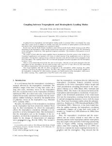
Fig. 4. Mean tropospheric NO2 vertical-column errors (solid circles) as a function of cloud radiance fraction, based on SP2 data from 21 March 2005. Vertical lines show error standard deviations and open circles indicate median values. Fig. 3. Histograms of the difference between estimated and original stratospheric NO2 columns over masked (polluted) areas based on simulated-data retrievals for January, March, July, and October 2005. Each histogram has a 2-sigma level deviation of approximately 0.2 × 1015 cm−2 . A

trop the CTM tropospheric vertical column, (2) σStrop are a priori Strop errors due to Atrop , and (3) σδVstrat are stratospheric interpolation errors in the masked regions (see Sect. 4.1.2). We write the combined variance as

A

trop (σVstrat )2 = (σSCTM /Astrat )2 + (σStrop /Astrat )2 + (σδVstrat )2 . trop

(22)

Although the CTM errors are not known, we estimate the uncertainties from sources (1) and (2) (first two terms) to be approximately 50 %. Therefore, by Eq. (10), with ε = 0.3 × 1015 cm−2 , these errors are − (< Strop > −< Strop >)/Astrat ,

4.1

Retrieval effects of a priori assumptions in the STS algorithm

The a priori tropospheric NO2 columns and the masking, interpolation, and smoothing components of the STS algorithm affect NO2 retrieval accuracy. In general, over the cleanest areas (open-ocean and high-latitude regions), the SP2 algorithm yields Vstrat values that are approximately as accurate as the NO2 slant columns and contain only small amounts of a priori model information from the tropospheric climatology. Relatively little independent tropospheric information is retrieved from these regions, but local enhancements relative to the a priori troposphere can be observed. The retrieval over clean regions consists of small-scale (smaller than ∼3◦ ) tropospheric features and measurement noise. Over polluted (masked) regions, the SP2 algorithm provides Vtrop retrievals that are mainly dependent on the assumed local profile shapes and surface reflectivity climatology via the air mass factors. Two scenarios in particular are challenging to the SP2 STS algorithm (and for nadir-viewing satellite retrievals in general). Firstly, over clean, unmasked regions, non-localized (broad) variations in tropospheric NO2 relative to the a priori climatology will necessarily appear as stratospheric NO2 . Secondly, in polluted, masked areas, stratospheric features that depart significantly from the mean stratosphere in surrounding unmasked areas will be aliased into the tropospheric column. For example, a small-scale stratospheric enhancement over a cloud-free polluted region on the US East Coast would be retrieved as a tropospheric enhancement. The inherent ambiguity in these scenarios can not be resolved without additional information about the partitioning of stratospheric and tropospheric NO2 . To examine the behavior of the STS algorithm under such conditions, we consider idealized, noise-free retrievals over unmasked and masked regions. These are discussed and illustrated in Sects. 4.1.1–4.1.3. For our simulations, we assume that the “true” stratospheric air mass factor, Astrat , is equal to its a priori estimate, Astrat , and is invariant on scales smaller than the widths of the smoothing windows: ≈ Astrat (on this scale we ignore the effects of viewing geometry). In this discussion, we use an overline for variables to represent “true” (as opposed to a priori) atmospheric values, brackets to indicate window averages, and a prime ( 0 ) to designate values in masked (polluted) areas.


2617

(25)

where < Vstrat > is the window-averaged true stratospheric vertical column. Equation (25) states that the retrieved stratospheric vertical column is the average of the true stratospheric vertical column plus an error term from the difference between the true and a priori tropospheric slant columns. When the a priori tropospheric slant column is correct and the true stratospheric field is smooth on the scale of the smoothing window, then the stratospheric retrieval is unbiased: Vstrat_RET ≈ Vstrat . If the true stratospheric field is homogeneous within the averaging window from Eq. (11), then the retrieved troposphere in unmasked regions is Vtrop_RET = Vtrop · (Atrop /Atrop ) + (< Strop > −< Strop >)/Atrop . (26)

When the a priori tropospheric air mass factors are accurate (Atrop ≈ Atrop ) and slowly varying, Eq. (26) becomes Vtrop_RET ≈< Vtrop > +(Vtrop − < Vtrop >).

(27)

Equation (27) shows that, in unmasked regions, the retrieved tropospheric vertical column is approximately equal to the a priori mean value (first term). However, the retrieval has additional fine-scale structure equal to the difference between the true tropospheric vertical column and its mean (second term). 4.1.2

Retrievals in masked (polluted) regions

The retrieved stratospheric vertical column in masked areas, 0 Vstrat_RET , is actually the interpolation-window average of the retrieved stratosphere in surrounding unmasked areas. We define the “true” stratosphere in masked areas as the similarly averaged true stratosphere from surrounding regions plus an amount, δVstrat , which varies from point to point inside the mask. The standard deviation of δVstrat is σδVstrat , which was derived in Sect. 3.2 from the histogram widths in Fig. 3. With these definitions, the tropospheric retrieval in a masked region can be shown to be 0 Vtrop_RET = V 0 trop · (A0 trop /A0trop ) +

(28)

(< Strop > −< Strop >)/A0trop + δVstrat · (A0strat /A0trop ), where A0strat and A0trop are the a priori stratospheric and tropospheric air mass factors in the masked area, and A0 trop is the true tropospheric air mass factor. As before, and < Strop > are the smoothed a priori and true tropospheric Atmos. Meas. Tech., 6, 2607–2626, 2013

2618


Fig. 5. NO2 vertical-column retrievals (red), using simulated data (black). The mean value of the tropospheric data (truth, black) was defined to be larger than that of the algorithm’s a priori troposphere (blue). Shown are nadir pixels along two orbital segments: (a) and (c) are stratosphere and troposphere, respectively, for an unmasked segment in the eastern Pacific; (b) and (d) are stratosphere and troposphere, respectively, for a masked segment over eastern North America. In these simulations, geolocation, viewing geometry, and cloud parameters were taken from two orbits on 21 March 2005.

slant columns, respectively, in the surrounding unmasked ar0 eas. We want our retrieval Vtrop_RET to be as close as possible to the true troposphere V 0 trop , and the three terms in Eq. (28) identify three possible sources of error. The first arises from potential mismatch of the true and a priori tropospheric air mass factors, A0 trop and A0trop . The true tropospheric vertical column will be scaled by their ratio. The second term shows errors due to the incorrect estimation of the a priori tropospheric slant columns in the surrounding areas. The third term describes tropospheric errors resulting from differences between the true stratosphere in the masked region and the mean stratosphere estimated from the surrounding regions. The second and third terms increase as the tropospheric air mass factor in the masked region (the denominator of each) decreases due to increasing aerosol or cloud fraction, for example. The result is that any biases caused by non-zero values for δVstrat or for – < Strop > outside the mask will be amplified as the cloud fraction for a given pixel inside the mask increases. The bias is bounded, because measurements with large cloud fractions generally switch to the unmasked case described in Sect. 4.1.1. 4.1.3

Examples using simulated data

Figure 5 shows retrievals of simulated OMI slant-column data. The plots represent nadir pixels along sections of two OMI orbits, with viewing geometry and cloud parameters taken from the orbital data. In this simulation, we assume that all a priori air mass factors are correct, i.e., the true Atmos. Meas. Tech., 6, 2607–2626, 2013

air mass factors are the same as those used in the retrieval. Figure 5a and c illustrate stratospheric and tropospheric retrievals, respectively, in an unmasked (clean) part of the eastern Pacific. The retrieved stratospheric vertical column (red curve in Fig. 5a) is biased high because the simulated tropospheric data were intentionally made 50 % larger than the a priori troposphere in the unmasked regions. This bias affects the retrieved stratosphere via the second term in Eq. (25). Figure 5c shows the corresponding tropospheric retrieval. As expected from Eq. (27), the retrieval (red) follows the a priori (blue) rather than the true data (black), on average. However, it is evident that some of the smaller-scale differential structure in the original data is preserved in the retrieval. Retrievals in a masked region of the Eastern US are shown in Fig. 5b and d. The differences between the true and retrieved stratospheres (Fig. 5c) are similar to the unmasked case (Fig. 5a), except that some regional variability is apparent. These deviations are due to intentional non-zero values of δVstrat used in constructing the stratospheric NO2 field. An example can be seen for the latitudes 30◦ N–37◦ N, where the stratospheric retrieval (interpolation from surrounding unmasked regions) underestimates the stratospheric data. The corresponding troposphere in the masked region is shown in Fig. 5d. Unlike the unmasked case, the retrieved troposphere here (red) is mostly independent of the a priori troposphere (blue) and is generally a good estimate of the true data (black). An obvious exception around 30◦ N–37◦ N latitude results from the previously noted stratospheric underestimation, which leads to a tropospheric overestimation.



2619

Fig. 6. Differences (= modified – nominal) in stratospheric field resulting from changes in masking threshold (nominal = 0.3 × 1015 cm−2 ) and interpolation window dimensions (see text) in the STS algorithm. (a) Tropospheric masking threshold decreased to 0.2 × 1015 cm−2 . (b) Masking threshold increased to 0.4 × 1015 cm−2 . (c) Interpolation window halved in latitude and longitude width relative to nominal size. (d) Interpolation window doubled in width.

Elsewhere, the tropospheric vertical column is slightly underestimated by an absolute amount comparable to that of the unmasked troposphere (Fig. 5c). As in the unmasked case, this underestimation is due to the error in the a priori troposphere for the clean regions. The relative effect in this case appears small, since overall tropospheric columns are much larger in the masked region (note the difference in y-axis scaling for Fig. 5c and d). In summary, the absolute stratospheric retrieval errors are generally small in most areas. The magnitude of the error depends on the magnitude of the bias between the a priori and true tropospheric fields. For OMI, we estimate that this bias introduces a stratospheric uncertainty of ∼0.2 × 1015 cm−2 or < 10 %. When tropospheric air mass factors are accurate, our simulations show that the absolute tropospheric verticalcolumn errors due to stratospheric errors are also small (on the order of 0.5 × 1015 cm−2 ) in both masked and unmasked regions. The corresponding relative tropospheric errors in unmasked regions may be large due to the small tropospheric background amounts in those regions. Errors in tropospheric air mass factors will lead to proportional increases in both the absolute and relative tropospheric vertical-column errors in all areas.

subtracted from the modified field. The results, shown in Fig. 6, suggest that the retrieval is fairly robust with respect to the threshold and window dimensions. In Fig. 6a, the masking threshold was reduced from its nominal value of 0.3 × 1015 cm−2 to 0.2 × 1015 cm−2 , and in Fig. 6b, the threshold was increased to 0.4 × 1015 cm−2 . The reduced threshold increases the number of masked pixels by a factor of ∼2, while the threshold increase approximately halves the masked-pixel count. The difference in the resultant Vstrat is generally smaller than 0.5 × 1015 cm−2 and is less than 0.1 × 1015 cm−2 over most of the Earth. The biggest effects are seen for the smaller threshold (0.2 × 1015 cm−2 ), since this threshold results in more than half of Northern Hemisphere pixels being masked, leaving little data from which to accurately interpolate the stratospheric field. Tests involving the interpolation algorithm are shown in Fig. 6c and d. In these figures, the latitude and longitude dimensions of the window were approximately halved and doubled, respectively. Results show that effects on the stratospheric field are even smaller than those seen in the threshold tests. We have also found that changing the shape of the interpolation function (e.g., from boxes to circles) makes a negligible difference in the resultant stratosphere.

4.1.4 Masking and interpolation sensitivity tests

4.2

The retrieved stratospheric field was examined for sensitivity to parameters that control the initial masking and interpolation in the STS algorithm. These steps are illustrated in Fig. 2d and e. We modified the masking threshold and the dimensions of the interpolation function (window) and computed the resultant stratospheric fields. In each case, the field based on the nominal parameters (see Sect. 2.4) was

Using NO2 slant columns from one day of OMI data for illustration, we compare SP2 retrievals with those from the SP1 algorithm (Bucsela et al., 2006) and the DOMINO v2 algorithm (Boersma et al., 2011). The retrieved stratospheric fields for one day are shown in Fig. 7, along with the GMI model field for the same date. The GMI stratosphere was


Comparisons with other NO2 retrieval algorithms and models

Atmos. Meas. Tech., 6, 2607–2626, 2013

2620


1

2 Fig. 7. Stratospheric NO2 vertical-column retrieval for the date 21 March 2005. (a) SP1. (b) SP2. (c) DOMINO. (d) GMI (scaled to the Figure 7: Stratospheric NO2factors). vertical column retrieval for the date 21 March 2005. (a) SP1. magnitude of 3SP2 using latitude-dependent scaling

4

(b) SP2. (c) DOMINO. (d) GMI (scaled to the magnitude of SP2 using latitude-dependent

5

scaling factors).

6 7 8 9 10

1 Fig. 8. Tropospheric NO2 vertical-column retrieval for the date 21 March 2005. (c) DOMINO. (d) GMI. Note that all 2 Figure 8: Tropospheric NO2 vertical column retrieval for(a) theSP1. date(b) 21SP2. March 2005. (a) SP1. negative values in SP1 were set to zero in the original SP1 public product. Also note that most of the negative values in the DOMINO (b) SP2. (c) DOMINO. (d) GMI. thatasall negative values in SP1 were set to zero in the product occur3 in cloudy or snow-covered regions and areNote flagged unreliable.

4

original SP1 public product. Also note that most of the negative values in the DOMINO

product occur in cloudy snow-covered regions and are flagged sampled at 5the OMI overpass time and or adjusted by empiramples are the as lowunreliable. SP1 stratospheric NO2 values in Westical scaling factors to give approximate agreement in magern Asia and the band of enhanced NO2 across the South6 nitude with the retrieved OMI stratosphere over the Pacific. ern US and parts of the Atlantic Ocean and North Sea. In The scaling7factors were assumed to be linear functions of some of these regions, the SP1 stratospheric values exceed latitude and to vary between about 1.1 and 1.4. Linear varithe values of Vinit (Fig. 2b), which should not occur, apart 46 ation was assumed for simplicity only – the actual ratio befrom measurement noise, since tropospheric NO2 amounts 8 tween the OMI and GMI stratospheres is more complicated, must be positive. Such artifacts are also evident in the v2 as evidenced by the discrepancy between the two stratoDOMINO stratospheric field over southern high latitudes, spheres (e.g., near the Equator). Nonetheless, a comparison the North Atlantic and parts of Siberia. Note the anomaof Fig. 7b and d shows that synoptic-scale structures in the lously high DOMINO stratospheric values in eastern Siberia model stratosphere are qualitatively similar to those retrieved associated with the breakup of the polar vortex (Dirksen et by the SP2 algorithm. The stratosphere of the SP1 retrieval al., 2011). DOMINO also shows stronger cross-track diurlacks structure on this scale and contains artifacts associnal variation in comparison to SP2 and Vinit (Fig. 2b). Troated with the wave-2 assumption in the SP1 retrieval. Expospheric retrievals for the same day in March are shown

Atmos. Meas. Tech., 6, 2607–2626, 2013



2621

Fig. 9. Monthly mean NO2 comparisons of SP1 (blue), SP2 (red), and DOMINO (green): (a) January stratospheric zonal mean, (b) July stratospheric zonal mean, (c) January NH troposphere (averaged over latitudes 35◦ N to 55◦ N), (d) July NH troposphere (averaged over latitudes 35◦ N to 55◦ N). In (c) and (d), the three regions of enhanced tropospheric NO2 represent, from left to right, the USA, Europe, and E. Asia, respectively. All measurements used for the tropospheric means were screened to exclude cloud radiance fractions greater than 50 %.

in Fig. 8. The tropospheric fields for all three OMI products (Fig. 8a, b, and c) are qualitatively similar to the GMI March monthly mean field shown in Fig. 8d. The SP1 field shown in Fig. 8a has been recomputed using an off-line version of the SP1 algorithm that retains any negative values of tropospheric NO2 . The SP2 tropospheric retrieval shows relatively few instances of negative tropospheric NO2 compared to the other two OMI products. Monthly means from January and July (not shown) indicate that approximately 8 to 9 % of Vtrop columns retrieved from SP2 are significantly negative, defined here as Vtrop < −0.2 × 1015 cm−2 . DOMINO tropospheric vertical columns have a somewhat higher frequency of negative values, and these occur predominantly in regions that are cloudy or snow-covered (and thus flagged as unreliable). Approximately 21 % of the mostly cloudy (cloud radiance fraction > 0.5) Vtrop retrievals from DOMINO are significantly negative, compared to ∼15 % of DOMINO retrievals in relatively cloud-free regions. A comparison of Figs. 7c and 8c shows that some of the negative tropospheric values in DOMINO are associated with the strong crosstrack variation in the DOMINO stratospheric field. Additional comparisons among the three OMI data products may be found in the Supplement. Maps are shown in Figs. S1– S5, and statistical comparisons in the form of PDFs are given in Fig. S6. The figures provide further evidence of the relative scarcity of negative tropospheric column amounts in SP2 compared to SP1 and DOMINO.


Larger-scale similarities and differences in the NO2 retrievals can be seen by examining monthly means. Figure 9 compares monthly zonal means of stratospheric NO2 in January and July from SP1, SP2 and DOMINO, and the longitudinal variation of monthly mean tropospheric NO2 in northern mid-latitudes for the same two months. In January and July, the stratospheric zonal means (Fig. 9a and b) are similar in all three products, with the SP2 slightly higher and the SP1 slightly lower than DOMINO. Larger differences are evident in the tropospheric means shown in Fig. 9c and d. Although the mean values of SP2 and DOMINO are similar (DOMINO is slightly lower in January and slightly higher in July at most longitudes), SP1 is consistently higher than SP2 by almost a factor of two in July. This discrepancy is likely due to the tropospheric air mass factors used in the SP1 retrieval, which did not account for the seasonal variability in NO2 profile shape (Lamsal et al., 2010). 4.3

Comparison with in situ measurements from INTEX-B

Validation of the OMNO2 SP2 is the subject of ongoing studies and will be covered in detail in a separate paper (Lamsal et al., 2013). Preliminary results suggest improved agreement with independent datasets for SP2 relative to SP1. The following example shows how NO2 from SP2 compares with data from the Intercontinental Chemical Transport Experiment (INTEX-B).

Atmos. Meas. Tech., 6, 2607–2626, 2013

2622


Fig. 10. Comparisons of tropospheric OMI NO2 retrievals vs. integrated in situ LIF NO2 measurements obtained during the INTEX-B field campaign over the Gulf of Mexico and clean Pacific locations. Shown are (a) SP1, but with collection 2 slant columns, (b) SP1 (current collection 3), and (c) SP2 (current collection 3). The solid line is an error-weighted least squares fit, and the dotted line is 1:1.

The INTEX-B campaign was conducted from March to May 2006 and included in situ data from the airborne LaserInduced Fluorescence (LIF) instrument (Thornton et al., 2000, 2003), which measured NO2 mixing ratios with an estimated accuracy of ±10 % or ±5ppt. Mixing-ratio profiles were obtained at a number of locations in and near the Gulf of Mexico and parts of the Pacific Ocean. The former region included land measurements at polluted locations near Mexico City and Houston. The LIF data were analyzed and compared by Bucsela et al. (2008), Boersma et al. (2008), and Hains et al. (2010) with OMI data. In the present study, we have employed a similar approach to that of Bucsela et al. (2008). LIF data were selected for analysis based on the cloud/aerosol amount, altitude range of the aircraft, and temporal (< 3 h) and spatial (< 20 km) proximity to the OMI overpass data. The profiles were integrated for comparison with OMI NO2 tropospheric columns. All profiles required extrapolation in altitude, both above and below the actual measurements, to cover the full tropospheric column, and the amount of extrapolation was accounted for in the uncertainties assigned to each profile. Comparisons with OMI were made using x- and y-error weighted linear regression. The following information describes our analysis of three different sets of OMNO2 data. The data are from (1) SP1 applied to collection 2 OMI data (as in the original study of Bucsela et al., 2008), (2) SP1 applied to collection 3, and (3) SP2 applied to collection 3. The collection 2 slant columns were retrieved from the OMI spectra based on pre-launch calibrations. Improved post-launch calibrations were used to construct a collection 3 dataset in 2007, as described by Dobber et al. (2008). All OMI examples shown previously in this study are based on collection 3 data. A summary of the comparison results is shown in Fig. 10. In general, the agreement between the LIF and OMI data is good in all cases. Figure 10a shows that the SP1 algorithm, using the original collection 2 OMI slant columns yields vertical columns slightly below those of the in situ LIF columns (see also Bucsela et

Atmos. Meas. Tech., 6, 2607–2626, 2013

al., 2008). The regression OMI vs. in situ yields slope = 0.9, y-intercept = 0.1 × 1015 cm−2 , and Pearson’s correlation coefficient r = 0.83. Using the collection 3 spectral radiances and the same SP1 algorithm (Fig. 10b), we obtain slope = 1.2, y-intercept = 0.2 × 1015 cm−2 , and r = 0.72, respectively. This result implies a modest overestimate of NO2 by OMI relative to the in situ measurements. Figure 10c shows the reanalysis of the same collection 3 data using the new SP2 algorithm. In this case, the slope and intercept are approximately unity and zero, respectively, and the correlation coefficient is r = 0.76. The slope and intercept in the latest OMNO2 dataset indicate the best agreement with the INTEX-B data of the three comparison figures. Although this analysis was based on springtime rather than summertime data, the smaller tropospheric columns in SP2 relative to SP1 (for the same collection 3 dataset) appear consistent with Fig. 9d and the results of Lamsal et al. (2013).

5

Summary and conclusions

The retrieval algorithm described in this paper represents an improvement on many previous and existing methods for retrieving NO2 vertical columns from nadir-viewing satellites. SP2 provides a more realistic, detailed stratosphere and troposphere and has a relatively small dependence on a priori information and assumptions. In the stratospheric retrieval, there is no assumption of global zonal invariance as in reference-sector methods, no assumption of wave-2 zonal variation as in SP1, no use of ancillary stratospheric limb measurements (e.g., Beirle et al., 2010), and no stratospheric CTM scaling or assimilation as employed in the OMI DOMINO product. The stratosphere computed in SP2 requires a monthly tropospheric climatology, but this is applied only to clean regions or to areas cloudy enough to effectively block the satellite’s view of tropospheric NO2 . Here the errors associated with the climatology are comparable to nominal measurement uncertainties in the stratosphere. In other regions, the stratosphere is interpolated with the introduction www.atmos-meas-tech.net/6/2607/2013/

E. J. Bucsela et al.: New NO2 retrieval algorithm for nadir-viewing satellite instruments of small additional errors in the stratospheric field. The effect on the retrieved stratosphere of modest changes in the interpolation parameters (e.g., the extent of masking or the interpolation-window size and shape) is relatively small. Tests using simulated data show reasonable accuracy in the OMI SP2 retrievals, with clear-sky tropospheric errors over most regions on the order of ∼1015 cm−2 . Recent validation studies comparing OMNO2 SP2 with independent measurements also suggest improvement over SP1-based validations. We note fewer instances of negative tropospheric vertical columns relative to SP1 and the DOMINO product. However, the general agreement between OMNO2 and DOMINO has improved with the introduction of the SP2 algorithm. This agreement is noteworthy, given the very different STS algorithms used in the two products. The discrepancies between polluted summertime tropospheric vertical columns from OMI and those from independent measurements have been greatly reduced in SP2 compared to SP1 and are also small relative to DOMINO. The quality of the SP2 data is currently being established by independent measurements in ongoing validation campaigns from ground, aircraft, and satellite instruments. Better error estimates in the SP2 product should facilitate the comparisons, and future work will help to refine the error estimates. Differences in the behavior of the SP2 algorithm under clear/cloudy, polluted/clean, and masked/unmasked conditions should also be kept in mind when comparing OMI datasets. Versions of the SP2 algorithm are also planned for testing with data from other satellite instruments, including SCIAMACHY, GOME-2 and TROPOMI. Supplementary material related to this article is available online at http://www.atmos-meas-tech.net/6/ 2607/2013/amt-6-2607-2013-supplement.pdf. Acknowledgements. We acknowledge the NASA Earth Science Division for funding of the OMI Standard NO2 product development and analysis. The Dutch-Finnish-built OMI instrument is part of the NASA EOS Aura satellite payload. The OMI instrument is managed by KNMI and the Netherlands Agency for Aerospace Programs (NIVR). The authors also wish to thank the editor and referees for their helpful comments in preparing this paper. Edited by: M. Weber

References Acarreta, J. R., deHaan, J. F., and Stammes, P.: Cloud pressure retrieval using the O2 -O2 absorption band at 477 nm, J. Geophys. Res., 109, D05204, doi:10.1029/2003JD003915, 2004. Bass and Johnsten, World Meteorological Organization, 1975. Beirle, S., Platt, U., von Glasow, R., Wenig, M., and Wagner, T.: Estimate of nitrogen oxide emissions from shipping by satellite remote sensing, Geophys. Res. Lett., 31, L18102, doi:10.1029/2004GL020312, 2004.


2623

Beirle, S., Kuhl, S., Pukite, J., and Wagner, T.: Retrieval of tropospheric column densities of NO2 from combined SCIAMACHY nadir/limb measurements, Atmos. Meas. Tech., 3, 283–299, doi:10.5194/amt-3-283-2010, 2010. Beirle, S., Boersma, K. F., Platt, U., Lawrence, M. G., and Wagner, T.: Megacity Emissions and Lifetimes of Nitrogen Oxides Probed from Space, Science, 333, 1737–1739, 2011. Bey, I., Jacob, D. J., Yantosca, R. M., Logan, J. A., Field, B. D., Fiore, A. M., Li, Q., Liu, H., Mickley, L. J., and Schultz, M. G.: Global modeling of tropospheric chemistry with assimilated meteorology: Model description and evaluation, J. Geophys. Res., 106, 23073–23095, 2001. Boersma, K. F., Bucsela, E. J., Brinksma, E. J., and Gleason, J. F.: NO2 , in: OMI Algorithm Theoretical Basis Document, 4, OMI Trace Gas Algorithms, ATB-OMI-04, Version 2.0, 20 edited by: Chance, K., 13–36, NASA Distrib. Active Archive Cent., Greenbelt, MD, USA, August 2002. Boersma, K. F., Eskes, H. J., and Brinksma, E. J.: Error analysis for tropospheric NO2 from space, J. Geophys. Res., 109, D04311, doi:10.1029/2003JD003962, 2004. Boersma, K. F., Eskes, H. J., Veefkind, J. P., Brinksma, E. J., van der A, R. J., Sneep, M., van den Oord, G. H. J., Levelt, P. F., Stammes, P., Gleason, J. F., and Bucsela, E. J.: Near-real time retrieval of tropospheric NO2 from OMI, Atmos. Chem. Phys., 7, 2103–2118, doi:10.5194/acp-7-2103-2007, 2007. Boersma, K. F., Jacob, D. J., Bucsela, E. J., Perring, A. E., Dirksen, R., van der A, R. J., Yantosca, R. M., Park, R. J., Wenig, M. O., Bertram, T. H., and Cohen, R. C.: Validation of OMI tropospheric NO2 observations during INTEX-B and application to constrain NOx emissions over the eastern United States and Mexico, Atmos. Environ., 42, 4480–4497, doi:10.1016/j.atmosenv.2008.02.004, 2008. Boersma, K. F., Eskes, H. J., Dirksen, R. J., van der A, R. J., Veefkind, J. P., Stammes, P., Huijnen, V., Kleipool, Q. L., Sneep, M., Claas, J., Leitão, J., Richter, A., Zhou, Y., and Brunner, D.: An improved tropospheric NO2 column retrieval algorithm for the Ozone Monitoring Instrument, Atmos. Meas. Tech., 4, 1905– 1928, doi:10.5194/amt-4-1905-2011, 2011. Bovensmann, H., Burrows, J. P., Buchwitz, M., Frerick, J., Noel, S., Chance, K. V., and Goede, A. P. H.: SCIAMACHY: Mission objectives and measurement modes, J. Atmos. Sci., 56, 127–150, 1999. Brewer, A. W., McElroy, C. T., and Kerr, J. B.: Nitrogen dioxide concentrations in the atmosphere, Nature, 246, 129–133, doi:10.1038/246129a0, 1973. Bucsela, E. J., Celarier, E. A., Wenig, M. O., Gleason, J. F., Veefkind, J. P., Boersma, K. F., and Brinksma, E. J.: Algorithm for NO2 vertical column retrieval from the Ozone Monitoring Instrument, IEEE Trans. Geosci. Remote Sens., 44, 1245–1258, 2006. Bucsela, E. J., Perring, A. E., Cohen, R. C., Boersma, K. F., Celarier, E. A., Gleason, J. F., Wenig, M. O., Bertram, T. H., Wooldridge, P. J., Dirksen, R., and Veefkind, J. P.: Comparison of tropospheric NO2 from in situ aircraft measurements with near-real-time and standard product data from OMI, J. Geophys. Res., 113, D16S31, doi:10.1029/2007JD008838, 2008. Burrows, J. P., Weber, M., Buchwitz, M., Rosanov, V. V., Ladstatter, A., Weissenmayer, A., Richter, A., DeBeek, R., Hoogen, R., Bramstedt, K., and Eichmann, K. U.: The Global Ozone Moni-

Atmos. Meas. Tech., 6, 2607–2626, 2013

2624


toring Experiment (GOME): Mission concept and first scientific results, J. Atmos. Sci., 56, 151–175, 1999. Callies, J., Corpaccioli, E., Eisinger, M., Hahne, A., and Lefebvre, A.: GOME-2 – Metop’s Second Generation Sensor for Operational Ozone Monitoring, ESA Bulletin, 102, 28–36, 2000. Castellanos, P. and Boersma, K. F.: Reductions in nitrogen oxides over Europe driven by environmental policy and economic recession, Scientific Reports, 2, 265, doi:10.1038/srep00265, 2012. Chance, K. V. and Spurr, R. J. D.: Ring effect studies: Rayleigh scattering, including molecular parameters for rotational Raman scattering, and the Fraunhofer spectrum, Appl. Optics, 36, 5224– 5230, doi:10.1364/AO.36.005224, 1997. Choi, Y., Wang, Y., Zeng, T., Cunnold, D., Yang, E.-S., Martin, R. V., Chance, K., Thouret, V., and Edgerton, E.: Springtime transitions of NO2 , CO, and O3 over North America: model evaluation and analysis, J. Geophys. Res. 113, D20311, doi:10.1029/2007JD009632, 2008. Davé, J. V.: Multiple scattering in a non-homogeneous, Rayleigh atmosphere, J. Atmos. Sci., 22, 273–279, 1965. Dirksen, R. J., Dobber, R. M., Voors, R., and Levelt, P. F.: Prelaunch characterization of the Ozone Monitoring Instrument transfer function in the spectral domain, Appl. Optics, 45, 3972–3981, doi:10.1364/AO.45.003972, 2006. Dirksen, R. J., Boersma, K. F., Eskes, H. J., Ionov, D. V., Bucsela, E. J., Levelt, P. F., and Kelder, H. M.: Evaluation of stratospheric NO2 retrieved from the Ozone Monitoring Instrument: Intercomparison, diurnal cycle, and trending J. Geophys. Res. 116, D08305, 2011doi:10.1029/2010JD014943, 2011. Dobber, M. R., Kleipool, Q., Dirksen, R., Levelt, P. F., Jaross, G., Taylor, S., Kelly, T., Flynn, L., Leppelmeier, G., and Rozemeijer, N.: Validation of Ozone Monitoring Instrument level-1b data products, J. Geophys. Res., 113, D15S06, doi:10.1029/2007JD008665, 2008. Douglass A. R., Stolarski, R. S., Strahan, S. E., and Connell, P. S.: Radicals and reservoirs in the GMI chemistry and transport model: Comparison to measurements, J. Geophys. Res., 109, D16302, doi:10.1029/2004JD004632, 2004. Duncan, B. N., Strahan, S. E., Yoshida, Y., Steenrod, S. D., and Livesey, N.: Model study of the cross-tropopause transport of biomass burning pollution, Atmos. Chem. Phys., 7, 3713–3736, doi:10.5194/acp-7-3713-2007, 2007. Finlayson-Pitts, B. J. and Pitts Jr., J. N.: Chemistry of the Upper and Lower Atmosphere, Academic Press, ISBN 012257060X, 1999. Frost, G. J., McKeen, S. A., Trainer, M., Ryerson, T. B., Neuman, J. A., Roberts, J. M., Swanson, A., Holloway, J. S., Sueper, D. T., Fortin, T., Parrish, D. D., Fehsenfeld, F. C., Flocke, F., Peckham, S. E., Grell, G. A., Kowal, D., Cartwright, J., Auerbach, N., and Habermann, T.: Effecs of changing power plant NOx emissions on ozone in the eastern United States: Proof of concept, J. Geophys. Res., 111, D12306, doi:10.1029/2005JD006354, 2006. Hains, J. C., Boersma, K. F., Kroon, M., Dirksen, R. J., Cohen, R. C., Perring, A. E., Bucsela, E. J., Volten, H., Swart, D. P. J., Richter, A., Wittrock, F., Schoenhardt, A., Wagner, T., Ibrahim, O. W., Van Roozendael, M., Pinardi, G., Gleason, J. F., Veefkind, J. P., and Levelt, P. F.: Testing and improving OMI DOMINO tropospheric NO2 using observations from the DANDELIONS and INTEX-B validation campaigns, J. Geophys. Res., 115, D05301, doi:10.1029/2009JD012399, 2010.

Atmos. Meas. Tech., 6, 2607–2626, 2013

Harder, J. W. and Brault, J. W.: Atmospheric measurements of water vapor in the 442-nm region, J. Geophys. Res., 102, 6245–6252, doi:10.1029/96JD01730, 1997. Heckel, A., Kim, S.-W., Frost, G. J., Richter, A., Trainer, M., and Burrows, J. P.: Influence of low spatial resolution a priori data on tropospheric NO2 satellite retrievals, Atmos. Meas. Tech., 4, 1805–1820, doi:10.5194/amt-4-1805-2011, 2011. Hilboll, A., Richter, A., Rozanov, A., Hodnebrog, Ø., Heckel, A., Solberg, S., Stordal, F., and Burrows, J. P.: Improvements to the retrieval of tropospheric NO2 from satellite – stratospheric correction using SCIAMACHY limb/nadir matching and comparison to Oslo CTM2 simulations, Atmos. Meas. Tech., 6, 565–584, doi:10.5194/amt-6-565-2013, 2013. Jaeglé, L., Steinberger, L., Martin, R. V., and Chance, K.: Global partitioning of NOx sources using satellite observations: Relative roles of fossil fuel combustion, biomass burning and soil emissions, Faraday Discuss., 130, 407–423, doi:10.1039/b502128f, 2005. Kim, S.-W., Heckel, A., McKeen, S. A., Frost, G. J., Hsie, E.-Y., Trainer, M. K., Richter, A., Burrows, J. P., Peckham, S. E., and Grell, G. A.: Satellite-observed U.S. power plant NOx emission reductions and their impact on air quality. Geophys. Res. Lett., 33, L22812, doi:10.1029/2006GL027749, 2006. Kleipool Q. L., Dobber, M. R., de Haan, J. F., and Levelt, P. F.: Earth surface reflectance climatology from 3 years of OMI data, J. Geophys. Res., 113, D18308, doi:10.1029/2008JD010290, 2008. Koelemeijer, R. B. A.,. De Haan, J. F, and Stammes, P.: A database of spectral surface reflectivity in the range 335–772 nm derived from 5.5 years of GOME observations, J. Geophys. Res., 108, D24070, doi:10.1029/2002JD002429, 2003. Lamsal, L. N., Martin, R. V., van Donkelaar, A., Celarier, E. A., Bucsela, E. J., Boersma, K. F., Dirksen, R., Luo, C., and Wang, Y.: Indirect validation of tropospheric nitrogen dioxide retrieved from the OMI satellite instrument: Insight into the seasonal variation of nitrogen oxides at northern midlatitudes, J. Geophys. Res., 115, D05302, doi:10.1029/2009JD013351, 2010. Lamsal, L. N.: Evaluation of improved operational standard tropospheric NO2 retrievals from Ozone Monitoring Instrument using in situ and surface-based NO2 observations, in preparation, 2013. Lin, J.-T., McElroy, M. B., and Boersma, K. F.: Constraint of anthropogenic NOx emissions in China from different sectors: a new methodology using multiple satellite retrievals, Atmos. Chem. Phys., 10, 63–78, doi:10.5194/acp-10-63-2010, 2010. Leue, C., Wenig, M., Wagner, T., Klimm, O., Platt, U., and Jähne, B.: Quantitative analysis of NOx emissions from Global Ozone Monitoring Experiment satellite image suences, J. Geophys. Res. 106, 5493–5505, 2001. Levelt, P. F., Hilsenrath, E., Leppelmeier, G. W., van den Oord, G. B. J., Bhartia, P. K., Tamminen, J., de Haan, J. F., and Veefkind ,J. P.: Science Objectives of the Ozone Monitoring Instrument, IEEE Trans Geo. Rem. Sens., 44, 1199–1208, doi:10.1109/TGRS.2006.872333, 2006. Lin, J.-T., McElroy, M. B., and Boersma, K. F.: Constraint of anthropogenic NOx emissions in China from different sectors: a new methodology using multiple satellite retrievals, Atmos. Chem. Phys., 10, 63–78, doi:10.5194/acp-10-63-2010, 2010. Martin, R. V., Chance, K., Jacob, D. J., Kurosu, T. P., Spurr, R. J. D., Bucsela, E., Gleason, J., Palmer, P. I., Bey, I., Fiore, A. M., Li, Q., Yantosca, R. M., and Koelmeijer, R. B. A.: An improved retrieval


E. J. Bucsela et al.: New NO2 retrieval algorithm for nadir-viewing satellite instruments of tropospheric nitrogen dioxide from GOME, J. Geophys. Res., 107, 4437, doi:10.1029/2001JD001027, 2002a. Martin, R. V., Jacob, D. J., Logan, J. A., Bey, I., Yantosca, R. M., Staudt, A. C., Li, Q., Fiore, A. M., Duncan, B. N., Liu, H., Ginoux, P., and Thouret, V.: Interpretation of TOMS observations of tropical tropospheric ozone with a global model and in situ observations, J. Geophys. Res., 107, 4351, doi:10.1029/2001JD001480, 2002b. Martin, R. V., Jacob, D. J., Chance, K., Kurosu, T. P., Palmer, P. I., and Evans, M. J.: Global inventory of nitrogen oxide emissions constrained by space-based observations of NO2 columns, J. Geophys. Res, 108, 4537, doi:10.1029/2003JD003453, 2003. Martin, R. V., Sioris, C. E., Chance, K. V., Ryerson, T. B., Bertram, T. H., Woolridge, P. J., Cohen, R. C., Neuman, J. A., Swanson, A., and Flocke, F. M.: Evaluation of space-based constraints on nitrogen oxide emissions with regional aircraft measurements over and downwind of eastern North America, J. Geophys. Res., 111, D15308, doi:10.1029/2005JD006680, 2006. Martin, R. V., Sauvage, B., Folkins, I., Sioris, C. E., Boone, C., Bernath, P., and Ziemke, J.: Space-based constraints on the production of nitric oxide by lightning, J. Geophys. Res., 112, D09309, doi:10.1029/2006JD007831, 2007. Noxon, J. F.: Nitrogen dioxide in the stratosphere and troposphere measured by ground-based absorption spectroscopy, Science, 189, 4202, 547–549, 1975. Palmer, P. I., Jacob, D. J., Chance, K., Martin, R. V., Spurr, R. J. D., Kurosu, T. P., Bey, I., Yantosca, R., and Fiore, A.: Air mass factor formulation for spectroscopic measurements from satellites: Application to formaldehyde retrievals from the Global Ozone Monitoring Experiment, J. Geophys. Res., 106, 14539–14550, doi:10.1029/2000JD900772, 2001. Platt, U.: Differential optical absorption spectroscopy (DOAS), edited by: Sigrist, M. W., in: Air Monitoring by Spectrometric Techniques, volume 127 of Chemical Analysis Series, 27–84, John Wiley, New York, USA, 1994. Platt, U. and Perner, D.: Measurements of atmospheric trace gases by long path differential UV/visible absorption spectroscopy, in: Optical and Laser Remote Sensing, edited by: Killinger, D. A. and Mooradien, A., 95–105, Springer Verlag, New York, USA, 1983. Platt, U. and Stutz, J.: Differential Optical Absorption Spectroscopy (DOAS), Principle and Applications, Springer Verlag Heidelberg, ISBN 3-340-21193-4, 2006. Richter, A. and Burrows, J. P.: Tropospheric NO2 from GOME measurements, Adv. Space Res., 29, 1673–1683, doi:10.1016/S02731177(02)00100-X, 2002. Richter, A., Burrows, J. P., Nüß, H., Granier, C., and Niemeier, U.: Increase in tropospheric nitrogen dioxide over China observed from space, Nature, 437, 129–132, 2005. Rienecker, M. M., Suarez, M. J., Todling, R., Bacmeister, J., Takacs, L., Liu, H. C., Gu, W., Sienkiewicz, M., Koster, R. D., Gelaro, R., Stajner, I., and Nielsen, J. E.: The GEOS-5 Data Assimilation System-Documentation of Versions 5.0.1, 5.1.0, and 5.2.0 Technical Report Series on Global Modeling and Data Assimilation, v27, 2008. Russell, A. R., Valin, L. C., Bucsela, E. J., Wenig, M. O., and Cohen, R. C.: Space-based Constraints on Spatial and Temporal Patterns of NOx Emissions in California, 2005−2008, Environ. Sci. Technol., 44, 3608–3615, doi:10.1021/es903451j, 2010.


2625

Russell, A. R., Perring, A. E., Valin, L. C., Bucsela, E. J., Browne, E. C., Wooldridge, P. J., and Cohen, R. C.: A high spatial resolution retrieval of NO2 column densities from OMI: method and evaluation, Atmos. Chem. Phys., 11, 8543–8554, doi:10.5194/acp-11-8543-2011, 2011. Schaub, D., Brunner, D., Boersma, K. F., Keller, J., Folini, D., Buchmann, B., Berresheim, H., and Staehelin, J.: SCIAMACHY tropospheric NO2 over Switzerland: estimates of NOx lifetimes and impact of the complex Alpine topography on the retrieval, Atmos. Chem. Phys., 7, 5971–5987, doi:10.5194/acp-7-5971-2007, 2007. Schoeberl, M. R., Douglass, A. R., Hlsenrath, E., Bhartia, P. K., Beer, R., Waters, J. W., Gunson, M., Froidevaux, L., Gille, J., Barnett, J., Levelt, P. F., and Decola, P.: Overview of the EOS Aura Mission, IEEE Trans. Geosci. Remote Sens., 44, 1066– 1074, 2006. Schumann, U. and Huntrieser, H.: The global lightning-induced nitrogen oxides source, Atmos. Chem. Phys., 7, 3823–3907, doi:10.5194/acp-7-3823-2007, 2007. Seinfeld, J. H. and Pandis, S. N.: Atmospheric Chemistry and Physics: From air pollution to climate change, John Wiley & Sons Inc, New York, 234–330, 1998. Sneep, M., De Haan, J., Stammes, P., Wang, P., Vanbauce, C., Joiner, J., Vasilkov, A. P., and Levelt, P. F.: Three way comparison between OMI/Aura and POLDER/PARASOL cloud pressure products, J. Geophys. Res., 113, D15S23, doi:10.1029/2007JD008694, 2008. Solomon, S. and Garcia, R. R.: On the distribution of long-lived tracers and chlorine species in the middle atmosphere, J. Geophys. Res., 89, 11633-11644, 1984. Stammes, P., Sneep, M., de Haan, J. F., Veefkind, J. P., Wang, P., and Levelt, P. F.: Effective cloud fractions from the Ozone Monitoring Instrument: Theoretical framework and validation, J. Geophys. Res., 113, D16S38, doi:10.1029/2007JD008820, 2008. Strahan, S. E., Duncan, B. N., and Hoor, P.: Observationally derived transport diagnostics for the lowermost stratosphere and their application to the GMI chemistry and transport model, Atmos. Chem. Phys., 7, 2435–2445, doi:10.5194/acp-7-2435-2007, 2007. Thornton, J. A., Wooldridge, P. J., and Cohen, R. C.: Atmospheric NO2 : In situ laser-induced fluorescence detection at parts per trillion mixing ratios, Anal. Chem., 72, 528–539, 2000. Thornton, J. A., Wooldridge, P. J., Cohen, R. C., Williams, E. J., Hereid, D., Fehsenfeld, F. C., Stutz, J., and Alicke, B.: Comparisons of in situ and long path measurements of NO in urban plumes, J. Geophys. Res., 108, 4496, doi:10.1029/2003JD003559, 2003. Tie, X., Zhang, R., Brasseur, G., and Lei, W.: Global: NOx production by lightning, J. Atmos. Chem., 43, 61–74, 2002. Valks, P. and Loyola, D.: Algorithm theoretical basis document for GOME-2 total column products of ozone, minor trace gases, and cloud properties. Technical Report, DLR/GOME-2/ATBD/01, Iss.1/C, http://www.wdc.dlr.de/sensors/gome2/DLR_GOME-2_ ATBD_1C, 2008. Valks, P., Pinardi, G., Richter, A., Lambert, J.-C., Hao, N., Loyola, D., Van Roozendael, M., and Emmadi, S.: Operational total and tropospheric NO2 column retrieval for GOME-2, Atmos. Meas. Tech., 4, 1491–1514, doi:10.5194/amt-4-1491-2011, 2011.

Atmos. Meas. Tech., 6, 2607–2626, 2013

2626


Vandaele, A. C., Hermans, C., Simon, P. C., Carleer, M., Colin, R., Fally, S., Mérienne, M. F., Jenouvrier, A., and Coquart, B.: Measurements of the NO2 absorption cross-section from 42 000 cm−1 to 10 000 cm−1 (238–1000 nm) at 220 K and 294 K, J. Quant. Spectrosc. Radiat. Transf., 59, 171–184, 1998. Velders, G. J. M., Granier, C., Portmann, R. W., Pfeilsticker, K., Wenig, M., Wagner, T., Platt, U., Richter, A., and Burrows, J. P.: Global tropospheric NO2 column distributions: Comparing three-dimensional model calculations with GOME measurements, J. Geophys. Res., 106, 12643–12660, 2001. Wenig, M. O., Cede, A. M., Bucsela, E. J., Celarier, E. A., Boersma, K. F., Veefkind, J. P., Brinksma, E. J., Gleason, J. F., and Herman, J. R.: Validation of OMI tropospheric NO2 column densities using direct-sun mode Brewer measurements at NASA Goddard Space Flight Center, J. Geophys. Res., 113, D16S45, doi:10.1029/2007JD008988, 2008.

Atmos. Meas. Tech., 6, 2607–2626, 2013

Zhang, Q., Streets, D. G., He, K., Wang, Y., Richter, A., Burrows, J. P., Uno, I., Jang, C. J., Chen, D., Yao, Z., and Lei, Y.: NOx emission trends for China, 1995–2004: The view from the ground and the view from space, J. Geophys. Res., 112, D22306, doi:10.1029/2007JD008684, 2007.


A new stratospheric and tropospheric NO2 retrieval algorithm for nadir ...

A new stratospheric and tropospheric NO2 retrieval algorithm for nadir ...

Suggest Documents

Tropospheric and stratospheric BrO and NO2 ... - ESA Earth Online

An improved tropospheric NO2 retrieval for OMI ... - Atmos. Meas. Tech

Retrieval and analysis of stratospheric NO2 from the ... - CiteSeerX

Retrieval of stratospheric O3 and NO2 profiles ... - odin-osiris.usask.ca

A new tropospheric and stratospheric Chemistry and ... - CiteSeerX

An improved retrieval of tropospheric NO2 from ... - Atmos. Meas. Tech

An improved retrieval of tropospheric NO2 from ... - Atmos. Meas. Tech

A new regularized inversion method for the retrieval of stratospheric ...

Stratospheric variability and tropospheric ozone - UCI ESS

Coupling between Tropospheric and Stratospheric ... - AMS Journals

Lower-Stratospheric and Upper-Tropospheric Disturbances Observed

Contrasting meridional structures of stratospheric and tropospheric ...

An Improved Total and Tropospheric NO2 Column Retrieval for GOME-2

SCIA Nadir observations of NO2 and BrO - IUP

Tropospheric NO2 variability over the metropolitan ...

Measurements of Tropospheric NO2 in Romania ... - BioMedSearch

Stratospheric Influences on Tropospheric Weather Systems

Stratospheric influences on the tropospheric seasonal ... - CiteSeerX

A NEW WIND VECTOR RETRIEVAL ALGORITHM FOR OCEANSAT-2 ...

A New Algorithm for the Satellite-Based Retrieval ... - Semantic Scholar

BOREAS - a new MAX-DOAS profile retrieval algorithm for aerosols

A stratospheric NO2 climatology from Odin/OSIRIS limb-scatter ...

Quantitative bias estimates for tropospheric NO2 columns ... - Tue

Inter-comparison of stratospheric O3 and NO2 abundances retrieved ...