ity to obtain improvements using outliers and a simple local search method. .... Outlier. Search with. Free islands. Events to. Speciation. Unused island criterion.
A Niche for Parallel Island Models: Outliers and Local Search Steven Gustafson and Edmund K. Burke School of Computer Science & IT University of Nottingham, UK {smg, ekb}@cs.nott.ac.uk Abstract This paper reports on the development of a novel island model for evolutionary algorithms, which is intrinsically parallel and intended to better utilise resources and outlier solutions encountered during search. Outliers serve as seeds for new islands using a similar evolutionary algorithm or a local search procedure. In this initial study, we examine a definition of outliers and demonstrate the ability to obtain improvements using outliers and a simple local search method.
1 Introduction Parallel models are typically used in evolutionary algorithms (EAs) to foster distributed computing. Sequential EAs can be easily converted to work in parallel, and these new parallel algorithms can be tuned to behave in a similar manner to their sequential counter-parts. The original island model in EAs [1] was motivated by a biological theory suggesting that isolated subpopulations encouraged speciation events [2]. The metaphor of speciation is often touched upon in the EA literature, but the island model is not the ubiquitous implementation of that metaphor. Instead, the meaning and motivation of the island model is blurred with other forms of distributed computing, for example grid topologies, multipopulation models and demes. This paper develops a model, briefly introduced in [3], that describes a niche for island models based on the metaphor of speciation. Specifically, we aim to better utilise outlier solutions, which potentially represent local optima, that are lost due to population convergence to other solutions. Populations in EAs contain dissimilar local optima at different stages of the search process. Without a deeper understanding of the representation, operators and fitness function, we do not know how these local optima, being in the same population, will affect search. As such, it is not unrealistic to believe that in many instances, good local optima are lost as the population converges to some other
optimum. We briefly describe evidence for such behaviour from the genetic programming (GP) search process in the following section. We survey several island model implementations from the EA literature, mainly using GP or a genetic algorithm (GA). The proposed parallel island model is then described in more detail, followed by an empirical study aimed at assessing its feasibility.
2 Background In [3], we denoted solutions in the population with relatively good solution quality and high dissimilarity from the population as outliers. We measured the ability of the operator to produce good solutions using outliers. Using several common problem domains, the results showed that outliers were typically very poor at producing good solutions. However, infrequent events where outliers were far more successful than the rest of the population suggested that, under the right circumstances, the search process could be significantly improved by leveraging outliers more effectively. Thus, we were motivated to hypothesise in [3] that search may be improved by isolating outliers from the current population. The model was to speciate outliers to new subpopulations or islands where they would evolve in isolation. That is, we would conduct a separate, possibly populationbased, search with these fit and dissimilar solutions in parallel to the main EA search. Parallelisation is necessary as some islands will halt due to non-improvement, and then be restarted by another concurrently executing island’s speciation event or restarted from previously archived outlier solutions. In this paper, we begin to validate this model. We use a tunably difficult problem and a wide range of easy to hard instances [4] for a canonical GP system. Initially, we aim to validate two principles of the model: 1. Examine a definition of outliers, and 2. Verify that a simple hill-climbing or local search method on outliers can improve the overall solution quality of the EA run.
Next, we look at previous examples of island models. Specifically, we focus on novel models that touch upon the concept of species. The island model is an example of a distributed population model where subpopulations are isolated during selection, breeding and evaluation. Islands typically focus the evolutionary process within subpopulations before migrating individuals to other islands, or conceptual processors, which also carry out an evolutionary process. At predetermined times during the search process, islands send and receive migrants to other islands. There are many variations of distributed models, e.g. islands, demes, and niching methods, where each requires numerous parameters to be defined and tuned. Some early examples of island models follow. In [5], a distributed model used the concept of a species representing several types that are capable of mating and producing viable offspring. In [6], a parallel GA was implemented on a hypercube structure. Random migrant selection and replacement was first introduced in [1]. The idea that islands should consist of distinctly different environments was seen in later work, often for coevolution. In [7], an architecture was used to adaptively co-evolve components in a speciation model. Subpopulations represented separate species, which were required to contribute to the overall fitness to survive. An injection island GA in [8] divided the search space into hierarchical levels, where populations trained on more general tasks are injected into populations with more specific tasks. The cohort GA [9] was designed to combat premature convergence, in the form of “hitchhiking” by allowing higher fit individuals to reproduce first, where offspring are assigned to cohorts based on their fitness. In [10], an island model was used for recurrent neural network training that varied control parameters in each sub population. In [11], a multipopulation algorithm performed migration between subpopulations where individuals were redistributed to new subpopulations based on a speciation tree method that places genetically similar individuals together. A local GA was then run on each island for a number of generations to serve as an ‘intensification’ phase. Much of the effort in distributed models in GP focus on increasing efficiency or adding computational resources by means of parallelisation. A typical example is found in [12], where each processor is responsible for the fitness evaluation and breeding of a subpopulation. Island models in GP are often considered as another form of multipopulation model, and in [13], various control parameters for multipopulation models are systematically studied. Multiple populations were also examined for GP in [14]. Just as multipopulation, distributed and island models often overlap with their goals and implementations, other forms of selection can also implement concepts of species and isolated subpopulations. For example, structure fit-
ness sharing [15] was applied to genetic programming to encourage the parameter search (functions and terminals) over similar structures (trees). Negative correlation [16] was used for learning ensembles of neural networks, where populations were divided into species and a representative from each species was included in the ensemble. Negative correlation was also investigated for GP as a way to improve diversity and prevent premature convergence [17]. In [18], a “species conserving” GA defined species in a population using distance metric, where species “seeds” were individuals that were at least as fit or more fit than the rest of the species. These individuals were then “conserved”, or copied, into the next generation.
3 The Niche for Islands Island models are used for a wide variety of purposes. From simple distributed computing to more advanced concepts of niches and hierarchical learning, island models are a convenient metaphor for EAs. In some EAs, for example GP, a niche may exist for island models to be cast into an explicit role to provide substantial and consistent improvements to the search process. The benefit of explicitly casting the island model for such a task is that is can allow for a more unified study and advancement of the method. Otherwise, the island model remains a general tool for diversity management, premature convergence avoidance, and efficient parallelisation – goals that are shared by diversity methods, selection techniques, specialised recombination operators and many distributed and multipopulation models, e.g. see [19]. The niche proposed in this paper is two-fold. Firstly, it is based on detecting solutions that are sufficiently different from the current population to contribute effectively to the search process, but that have good enough solution quality to be considered in some alternative search environment. The island in this case is a metaphor for a search process specifically designed for these solutions. For example, a simple local search method may be capable of improving solution quality. Or, a more complex populationbased method using outliers and specialised initialisation techniques may be better able to improve overall solution quality. Secondly, the proposed niche is based on a parallel algorithm capable of managing speciation events and resources to achieve maximum efficiency and search performance. The principles of the niche for island models are: 1. Solutions with good quality and an inability to contribute to search are speciated. 2. Speciation consists of allocating computational resources toward a new search process for these solutions.
Island at generation G
G+1
G+2 Search stopped due an improvement criterion
X
Initial population Speciation Events to Free islands
Search on island re−started based on speciation event
Search with Outlier Unused island
quality using local search. Note that, at this stage, we are not explicitly investigating the parallel aspects of the model. However, without first validating the aforementioned principles of the model, it is unlikely that the it will be successfull once parallelism is added. Next, we describe the Tree-String problem, the GP system and instances used in the study, the outlier definition and the local search method.
4.1 The Tree-String Problem
Unused island
X
Figure 1. Proposed island model evolutionary process with dynamic resource allocation.
3. Resources are used in parallel and managed dynamically. 4. Search processes are awarded more resources based on achieving improvements in overall solution quality. At this stage in the study of this proposed niche, we are mainly concerned with validating its components in a piecemeal fashion. In this way, we can assess each basic component independently to understand the model’s feasibility and the overall design. Figure 1 illustrates the proposed parallel island model where search on an island halts due to consecutive non-improvement events. Search on that island may be re-started due to another speciation event from another island. In this way, it is hoped that islands can not only leverage outlier solutions but also provide an efficient and simple way to perform dynamic resource allocation during the search process.
4 Experimental Verification We begin to study the proposed parallel island model by addressing the two points described in Section 2: Given a simple and intuitive definition of outliers [3], how many outliers are there in the population at different times, and can they be used to improve the overall solution quality than that which was achieved in the the run in which they occurred? To address this question, we carry-out experiments using the Tree-String problem, archive outliers found during the EA run, and conduct several local search methods with the archived outliers afterwards. Initially, we will simply look for improved solution quality, the number of outliers occurring at three different times during the search process and how successful they are at improving solution
The Tree-String problem is an artificial domain constructed to capture two important features of GP search: solution structure and content. This problem was briefly described in [3] and more thoroughly in [4]. The TreeString problem captures many elements of other artificial domains and has many similarities to other benchmark domains (as described along with some experimental evidence in [3]). The goal of the Tree-String problem is to derive specific structure and content elements simultaneously. Instances are defined using a target solution consisting of a tree shape and content. Candidate solutions are measured for their similarity to the target solution with respect to both tree shape and content. The Tree-String problem is defined as a tuple Π: Π = (Ψ, Ξ, t, α, γ, δ), where an instance is represented by a target solution t, composed of content elements from the set Ψ and has a tree shape defined by elements from the set Ξ. In this study, and in [4], we use the following: • Ξ = {n, l}, representing nodes and leaves in binary syntax trees, • Ψ = {A, . . . , D}, representing node and leaf labels, • α(t) �→ Ξ∗ , a breadth-first tree traversal over solution structure (tree shape) creating the structure string, • γ(t) �→ Ψ∗ , a depth-first, in-order tree traversal over solution content creating the content string, • δ(α(tt ), α(tc )) �→ i ∈ ℵ, and • δ(γ(tt ), γ(tc )) �→ j ∈ ℵ, where i and j represent the heuristic solution quality of tc compared to instance tt , and δ is the longest common substring function. A multiobjective Pareto criterion is used for fitness evaluation with the structure and content objectives, described in Section 4.6. In the Tree-String problem, as defined above, the portion of the solution that contributes to the structure objective is likely to be different from the part that contributes toward the content objective. This property is due to the use of the breadth-first traversal for the structure objective and the
Random Tree Shapes Selected Shapes τy
Tree Size
250 200
τ
150 100
6
τ 5 4 τ ττ3 τ2
50 τ
0 4
1
6
8
8
τ7
10
12
14
16
Tree Depth Trees selected with increasing depth
τ
1
τ
4
τ
7
τ
8
Trees selected with increasing size and same depth
Trees Selected and Tree Distribution 300
τ
6
τ
5
τ3
τ
2
Figure 2. The 500 tree shapes produced are plotted according to their depth and size (number of nodes).
depth-first traversal for the content objective. The fact that the two objectives are interdependent is likely to make it difficult for transformation operators to affect either content or structure objectives alone.
4.2 Tree-String Instances We create instances in the Tree-String problem with an increasing size (number of nodes) at the same depth, increasing size with increasing depths, and, over these shapes, increasing content alphabet size. These two features, tree size (across depths and within the same depth) and content size, are expected to lead to increased difficulty for GP. To create the set of tree shapes on which to place random content, forming an instance, we generate a tree shape using an iterative tree growth method. The method iteratively adds two child nodes to a probabilistically chosen leaf node, starting with the root. To produce 500 random trees with depths between 5 and 15, and with size between 15 and 272 nodes, we: (1) randomly pick a tree size from the latter range, and (2) iteratively grow a tree shape to that size with a limit of depth 15. The 500 random trees shapes created are shown in Figure 2 according to their depth and size. We select tree shapes from depths 7, 9, 11, and 13, labelled as τ 1,4,7,8 in Figure 2, respectively. These shapes are are chosen to be close to the mean size for that depth with the aim that tree shape alone will not affect difficulty. We also select tree shapes from depth 9 with increasing sizes, labelled as τ 2,3,5,6 in Figure 2, respectively. These trees are shown in Figure 2 using a circular lattice visualisation. The root node lies at the very center, and each two child nodes lie at the intersection of subsequent lines. The inner-ring marks the
maximum depth of that tree. The second step to define our instances is creating the content that each instance’s tree shape will have. To create instances that range in content difficulty, we create four random strings for each tree shape instance, where each random string uses an increasing number of symbols, starting with one. We denote the selected tree shape for an instance with τ y , and the number of symbols used to generate the y . Thus, we have random string with a subscript, i.e. τ(#Ψ) 1..8 instances defined in these ranges: τ1..4 . Note that the y in τ y denotes the tree shape selected from Figure 2. Each random string will be the same size as the tree shape under consideration - producing 4 × 8 instances. The GP system will use the same content set as used to create the current instance under consideration.
4.3 The GP System The GP algorithm is generational with a population size of 50. Two-parent subtree crossover is used to transform existing solutions into new ones. Two parent crossover selects a subtree (where non-leaf nodes are selected 90% of the time) from each parent and swaps them. All children are valid provided they are within a depth limit of 17. To select parents for crossover, tournament selection with a tournament size of 3 is used. The initial population is created by producing random trees using the Full and Grow methods equally between depths 2 and 4. A stopping criterion of 50 generations is used. Fitness is based on the two objectives of matching solution content and solution structure to a target instance content and structure, as described above. A Pareto criterion is used for selection, described in detail in Section 4.6. The GP method is run for 30 runs on each instance, creating 960 runs. We report the improvement of solution quality as the total size of the tree minus the longest common substring for structure and the total size minus the longest common substring for content. These values are normalised by the size of the target instance.
4.4 Instance Difficulty In Figure 3, some of the best quality solutions from each run are plotted. The Left hand graph in Figure 3 shows that as the content alphabet size increases, over all instances, improvements are made more in the structure objective. The Right hand graph of Figure 3 shows how the instances become harder for GP with increasing size, i.e. there is less overall improvement in both objectives. Note that for τ1y , GP is capable of meeting the optimal content objective, but it improves the structure objective to an even lesser degree. In summary, as expected, the tree shapes and content generation we selected created instances that range in difficulty
Size Difficulty - Best Fitness of Run 1
0.8
0.8
structure objective
structure objective
Content Difficulty - Best Fitness of Run 1
0.6
0.4
0.2
0
0.2
0.4 0.6 content objective
0.8
0.4
0.2
one two three four
0
0.6
a b c d
0 1
0
0.2
0.4 0.6 content objective
0.8
1
Figure 3. In the Left Figure, the instances are grouped according to their content alphabet size: one = τ11..8 , two = τ21..8 , three = τ31..8 , f our = τ41..8 . In the Right Figure, the instances are grouped 1,2 3,4 5,6 7,8 according to their increasing size: a = τ1..4 , b = τ1..4 , c = τ1..4 , d = τ1..4 . Only a sample of all data points are shown. Regression lines highlight the trends in the groupings.
Generation 15 - Outlier Contribution 50
Quartiles
40
4.5 Outliers and Survivability
30 20
In [3], we reported on the general inability of outliers to contribute consistently to the search process using one instance of the Tree-String problem and three common benchmark instances. We provide a brief analysis to support that conclusion for our study here. Using the results from our 32 instances and 960 runs, we count the number solutions with a pair-wise distance greater than the population’s mean pairwise distance and that have a better solution quality over more than half the population. Figure 4 (Left hand graph) shows a box and whiskers plot for the average number of these solutions (Outliers) in generation 15. We also count the average number of offspring these solutions produced (Produced in Figure 4), and then the average number of times those offspring were selected to produce an offspring in the following generation (Survived in Figure 4). Offspring produced by outliers tend to produce fewer offspring themselves, but with a surprisingly wide-range. These results can be expected when the population converges away from outlier solutions. These results also support the search behaviour of focusing less on dissimilar solutions with good quality. However, the wide-range of Survived in Figure 4, albeit heavily skewed toward 0, suggests that outliers are capable of providing significantly good solutions under some circumstances. The average distribution of pair-wise distances from all runs at generation 15 is shown in the Right hand graph of Figure 4. Note that in the above, outliers had a pair-wise distance greater than the population’s mean av-
Pair-wise Distances
Average Number
for GP with regard to improvement and with respect to solution content and structure.
10 0
9 8 7 6 5 4 3 2 1 0 0
Outliers
Produced
Survived
0.2
0.4 0.6 Dissimilarity
0.8
Figure 4. In the Left hand graph, the Number of Outliers at generation 15, number of offspring Produced by those outliers, and the number of those offspring that Survived to produce offspring in the next generation. The graph on the Right shows the distribution of pair-wise distances at generation 15.
erage pair-wise distance. In the study below, outliers are defined with a pair-wise distance greater than one standard deviation from the population’s mean distance. Using that definition, there are fewer outliers, as seen in Table 1, where virtually none Survived.
4.6 Outlier Definition We initially define outliers as genetically different from the rest of the population according to an edit distance. The edit distance is defined as follows: Two trees are overlapped at the root, and the number of node transformations, insertions and deletions that are required to make the two trees structurally and syntactically equal are counted. The dis-
tance is normalised by tree size. An individual’s pair-wise distance is the average of all the normalised distances to the rest of the population. This value is compared to the population’s mean pair-wise distance. A solution is an outlier if it is better than more than half of the population in quality (using a Pareto criterion, described next) and has a pair-wise distance greater than 1 standard deviation from the mean of the population’s average pair-wise distance. We initially archive outliers at generation 5, generation 15 and generation 30. Our definition of outliers is just one of many possible. Other definitions may be more suitable or appropriate. The Pareto criterion used for the outlier definition, and for selection in the GP algorithm, defines a solution as better than another if it is better in at least one objective and not worse in the other. Two solutions are equal, according to the Pareto criterion, if they are equal in both objectives or better and worse in the same number of objectives. Note that the solutions (Best of Run) shown in Figures 3 represent one (of possibly several) nondominated solutions that define the Pareto front for a run.
4.7 A Simple Local Searcher The local search method generates 10 solutions using subtree mutation from a given solution. Subtree mutation randomly creates a subtree between depth 1 and 3, using either the Full or Grow method, the same methods used to create the initial population. Subtree mutation then selects, with uniform probability, a node in the solution and replaces it with the new subtree. New solutions with better solution quality replace the current solution. We carry-out this procedure for 50 steps. We call a local search successful if it is able to produce a solution that is better-than the nondominated solution reported as the Best by the run from where the outlier came. For each outlier, we iterate the local search 10 times.
Table 1. The average number of outliers found in the 30 runs for each of the 32 instances at generation 5, 15 and 30. 10 local searches were perfomend with each outlier, the number of times (n) a better solution was found, and the percent of local searches that found a better solution, are also reported.
τxy x τ11 2 3 4
τ12 2 3 4
τ13 2 3 4
τ14 2 3 4
τ15 2 3 4
τ16 2 3 4
τ17 2 3 4
τ18 2 3
4.8 Results Table 1 shows the results for conducting the local search on outliers. Results for each instance are shown for the different content alphabet sizes (τx ). All instances had some runs which were improved by performing the local search on outliers. When the instances contained only the A symbol, local search was more effective. As instances became more difficult, fewer runs where improved. Table 1 also reports on the average number of outliers found at generation 5, 15 and 30. A population contained 50 solutions, and the definition of outliers resulted in around 5% of those being classified as outliers. There appeared to be slightly more, on average, outliers at generation 15. These numbers can change according to problems,
4
n 30
runs 25 1 7 9 24 10 14 8 21 11 14 13 17 5 10 9 18 6 4 6 12 9 9 9 17 9 8 7 3 10 6 8
Average #Outliers (Success %) gen. 5 gen. 15 gen. 30 0.77 (10.2%) 1.73 (6.7%) 2.10 (0.5%) 0.30 (0.0%) 1.53 (0.0%) 1.13 (0.0%) 0.13 (0.0%) 1.50 (0.0%) 1.27 (0.1%) 0.17 (0.0%) 1.27 (0.0%) 1.13 (0.0%) 0.77 (5.8%) 2.53 (10.0%) 2.17 (5.5%) 0.07 (0.1%) 1.60 (5.3%) 1.33 (0.0%) 0.07 (0.0%) 1.53 (0.0%) 1.47 (0.0%) 0.03 (0.0%) 1.43 (0.1%) 1.40 (0.0%) 0.90 (10.8%) 1.53 (10.7%) 1.37 (7.3%) 0.33 (1.0%) 1.40 (0.1%) 0.97 (10.0%) 0.07 (10.0%) 1.50 (0.2%) 1.60 (0.0%) 0.07 (0.1%) 1.63 (3.0%) 1.23 (10.0%) 0.67 (10.0%) 1.43 (1.0%) 1.23 (10.5%) 0.60 (0.1%) 1.13 (10.6%) 0.93 (0.0%) 0.13 (0.0%) 1.63 (0.0%) 1.37 (6.8%) 0.07 (0.0%) 1.37 (0.0%) 1.07 (0.1%) 1.03 (13.8%) 1.63 (51.2%) 1.03 (0.0%) 0.40 (0.3%) 2.07 (0.0%) 0.60 (0.0%) 0.03 (0.0%) 1.67 (0.0%) 0.90 (0.0%) 0.03 (0.0%) 1.20 (0.0%) 0.87 (0.2%) 1.10 (0.0%) 0.97 (10.0%) 0.90 (0.3%) 0.40 (10.0%) 1.63 (0.0%) 1.20 (0.0%) 0.30 (0.1%) 1.57 (0.1%) 0.90 (10.8%) 0.17 (20.0%) 1.63 (0.0%) 1.10 (0.0%) 1.20 (31.0%) 0.97 (0.5%) 0.53 (10.0%) 0.33 (0.0%) 1.07 (10.5%) 0.67 (0.0%) 0.13 (0.0%) 1.70 (0.0%) 0.80 (0.0%) 0.43 (0.0%) 1.30 (2.5%) 0.93 (0.1%) 0.83 (0.0%) 0.93 (0.0%) 0.23 (0.0%) 0.20 (0.0%) 1.87 (0.0%) 1.00 (0.0%) 0.17 (0.0%) 1.33 (0.3%) 0.93 (0.0%) 0.17 (0.0%) 1.67 (0.0%) 1.47 (0.0%)
instances and the method used for defining outliers. Note that in Figure 4, where outliers had a less strict dissimilarity requirement, the median number of outliers at generation 15 was around 15 out of the 50 solutions. Table 1 also reports the success rate of the local searches for improving the run’s solution quality. This is the percentage of the 10 local searches carried out for each outlier. Local searches for instances with τ1y , the easiest instances, were more successful at improving overall solution quality. In summary, to increase the likelihood of successful local searches, outliers should be taken from a variety
Nondominated solutions (one from each run) that were (and were not) Improved
structure objective
0.7 0.6 0.5 0.4 0.3 Improved Not Improved New Solutions
0.2 0.3
0.4
0.5 0.6 content objective
0.7
0.8
Figure 5. Represenative results from one instance: τ34 . The runs that were Improved, produced the New Solutions.
of times (generations) during the evolutionary search process to buffer against variations in instance difficulty. With respect to which runs were improved by local search, we show the results from a representative instance, τ34 , in Figure 5. The original runs that were improved by local search were generally not the best runs overall in solution quality. However, the new solutions produced by local search were often better or competitive with the best solutions from all runs. This simple local search on outliers provides a way to increase poorer GP runs to the same level and better than the best GP runs, possibly with better efficiency. We expect to see even better results with a slightly more sophisticated local search or outlier specific search method in future work.
of improving the run’s overall solution quality. Note that practically no algorithmic tuning was performed to achieve these results. It is also significant to note that these results were achieved using a wide range of instances ranging in two kinds of difficult, size and content and structure objectives. As we have verified the first goal of the proposed parallel island model (the possibility of speciating outliers), we will now address the ability of the model to efficiently allocate computational resources to speciation events, to manage resources efficiently and to detect non-improving searches. There are some other issues that we did not address in this study. For example, we did not test if any solution would lead to better solution quality using a local search method, or if the local search resulted in a similar kind of solution as that found by the EA run. Also, the type of search carried-out on an island was not investigated. We used a local search method here, but it is likely that seeding a new population using an outlier and conducting a standard EA search process would be a very efficient way to implement a multi-start EA algorithm. Future work will assess how efficient the local search method was and whether improved results can be achieved more efficiently using local search and outliers and a stopping criterion for the EA run. We will also look at using other search methods on the islands seeded with outliers. Our goal is to determine if a parallel island model using speciation can lead to improved solution quality using less computational resources than the standard EA run, and to provide some insight into the type of search procedure more suitable for outlier solutions. Regardless of the final verdict on our proposed model, we have demonstrated here the ability to achieve improved solution quality using outliers and local search.
5 Discussion
6 Conclusions
The study reported in this paper was aimed at addressing the concept of speciating solutions with good quality but that have an inability to normally contribute to the search process. We consider such solutions, based on earlier work[3] and some brief evidence reported here, to have a high amount of dissimilarity from the rest of the population and a relatively good fitness. Due to the typical amount of convergence in an EA run, we expected dissimilar solutions to be less able to consistently interact in a population-based search using multiple parent operators. As the EA search is concerned primarily with improving solution quality, we focus on dissimilar solutions that are also highly fit, or that represent potential local optima in the current population. To validate the concept of speciating solutions, we first archived outlier solutions and then carried out a simple local search procedure on them. These local searches are capable
This paper reported on the initial validation of a parallel island model for EAs. The proposed model is intended to fill a niche in EA search where good local optima (called outliers in this paper) are explicitly leveraged by a parallel search method. This parallel search method can be a population-based search, local search or some other suitable method. The island model is intended to dynamically manage resources by speciating the outliers to available resources. In this paper, we reported on the ability to detect outliers in GP and successfully conduct a simple local search method on them to improve overall solution quality. As the local search method was applied to solutions from early generations, it is very likely that search efficiency can also be improved. The experiments used a range of difficult instances on a problem designed to capture essential features from many commonly used and other artificial domains. The methodology and experimentation settings were
based on high level intuition and were not subjected to a large amount of tuning, making the results more likely to be generalisable. Acknowledgements: This work was supported by EPSRC grant GR/S70197/01.
References [1] J.P. Cohoon, S.U. Hegde, W.N. Martin, and D. Richards. Punctuated equilibria: a parallel genetic algorithm. In J.J. Grefenstette, editor, Proceedings of the Second International Conference on Genetic Algorithms, pages 148–154, Hillsdale, NJ, USA, 1987. Lawrence Erlbaum Associates. [2] N. Eldredge and S.J. Gould. Punctuated Equilibria: An Alternative to Phyletic Gradualism, chapter 5, pages 82–115. Freeman, Cooper and Co., 1972. [3] S. Gustafson. An Analysis of Diversity in Genetic Programming. PhD thesis, School of Computer Science and Information Technology, University of Nottingham, Nottingham, England, February 2004. [4] S. Gustafson, E.K. Burke, and N. Krasnogor. The treestring problem: An artificial domain for structure and content search. In M. Keijzer et al., editors, Genetic Programming, Proceedings of the 6th European Conference, volume 3447 of LNCS, pages 215–226, Lausanne, 2005. Springer-Verlag. [5] C. Pettey, M. Leuze, and J. Grefenstette. A parallel genetic algorithm. In J.J. Grefenstette, editor, Proceedings of the Second International Conference on Genetic Algorithms and Their Applications, Hillsdale, NJ, USA, 1987. Lawrence Erlbaum Associates. [6] R. Tanese. Parallel genetic algorithms for a hypercube. In J.J. Grefenstette, editor, Proceedings of the Second International Conference on Genetic Algorithms and Their Applications, pages 177–183, Hillsdale, NJ, USA, 1987. Lawrence Erlbaum Associates. [7] M.A. Potter and K.A. De Jong. Cooperative coevolution: An architecture for evolving coadapted subcomponents. Evolutionary Computation, 8(1):1–29, 2000. [8] S-C. Lin, W.F. Punch, and E.D. Goodman. Coarse-grain genetic algorithms, categorization and new approaches. In Sixth IEEE Symposium on Parallel and Distributed Processing, pages 28–37, Dallas, TX, USA, Oct 1994. IEEE Computer Society Press. [9] J.H. Holland. Building blocks, cohort genetic algorithms, and hyperplane-defined functions. Evolutionary Computation, 8(4):373–391, 2000. [10] P. Adamidis and V. Petridis. Co-operating populations with different evolution behavior. In Proceedings of 1996 IEEE International Conference on Evolutionary Computation, pages 188–191, Japan, May 1996. [11] M. Bessaou, A. P´etrowski, and P. Siarry. Island model cooperating with speciation for multimodal optimization. In M. Schoenauer et al., editors, Parallel Problem Solving from Nature, pages 437–446, Paris, France, 2000. Springer Verlag.
[12] D. Andre and J.R. Koza. Parallel genetic programming: A scalable implementation using the transputer network architecture. In P.J. Angeline and K.E. Kinnear, Jr., editors, Advances in Genetic Programing 2, chapter 16. The MIT Press, Cambridge, MA, USA, 1996. [13] F. Fernandez, M. Tomassini, and L. Vanneschi. An empirical study of multipopulation genetic programming. Genetic Programming and Evolvable Machines, 4(1):21–51, March 2003. [14] W.F. Punch, D. Zongker, and E.D. Goodman. The royal tree problem, a benchmark for single and multi-population genetic programming. In P.J. Angeline and K.E. Kinnear, Jr., editors, Advances in Genetic Programming 2, chapter 15, pages 299–316. The MIT Press, Cambridge, MA, USA, 1996. [15] J. Hu et al. Structure fitness sharing (SFS) for evolutionary design by genetic programming. In W.B. Langdon et al., editors, Proceedings of the Genetic and Evolutionary Computation Conference, pages 780–787, New York, 9-13 July 2002. Morgan Kaufmann Publishers. [16] Y. Liu, X. Yao, and T. Higuchi. Evolutionary ensembles with negative correlation learning. IEEE Transactions on Evolutionary Computation, 4(4):380–387, November 2000. [17] R. McKay and H.A. Abbass. Anti-correlation: A diversity promoting mechanisms in ensemble learning. The Australian Journal of Intelligent Information Processing Systems, (3/4):139–149, 2001. [18] J.-P. Li, M.E. Balazs, G.T. Parks, and P.J. Clarkson. A species conserving genetic algorithm for multimodal function optimization. Evolutionary Computation, 10(3):207– 234, 2002. [19] E.K. Burke, S. Gustafson, and G. Kendall. Diversity in genetic programming: An analysis of measures and correlation with fitness. IEEE Transactions on Evolutionary Computation, 8(1):47–62, 2004.