A nodal-based finite element approximation of the ... - Semantic Scholar

A nodal-based finite element approximation of the Maxwell problem suitable for singular solutions Santiago Badia

Ramon Codina Abstract

A new mixed finite element approximation of Maxwell’s problem is proposed, its main features being that it is based on a novel augmented formulation of the continuous problem and the introduction of a mesh dependent stabilizing term, which yields a very weak control on the divergence of the unknown. The method is shown to be stable and convergent in the natural H(curl; Ω) norm for this unknown. In particular, convergence also applies to singular solutions, for which classical nodal based interpolations are known to suffer from spurious convergence upon mesh refinement.

1 Introduction The simulation of electromagnetic phenomena with increasing complexity demands accurate and efficient numerical methods suitable for large-scale computing. Finite element (FE) methods are commonly used in this context because they can easily handle complicated geometries by using unstructured grids, provide a rigorous mathematical framework and allow adaptation. In many applications of current interest, the electromagnetic problem is coupled to other physical processes. Salient examples of multiphysics phenomena that include electromagnetics are magnetohydrodynamics and plasma physics. These two problems have experienced increasing attention due to the need to develop numerical laboratories in fusion technology design. The simulation of these problems (and many others) would benefit of an all-purpose FE method that would be suitable for the different subproblems at hand, simplifying the implementation issues and the enforcement of the coupling conditions. In particular, an all-purpose continuous nodal-based formulation would be a favored candidate. E.g. the Navier-Stokes equations are commonly solved with stabilized FE approximations that can deal with the singularly perturbed nature of the system for high Reynolds numbers and circumvent the restrictions related to the corresponding inf-sup condition (see e.g. [8, 9]). In plasma physics, fields computed by discontinuous FE Maxwell solvers create a considerable numerical noise when embedded in a plasma code, e.g. using the particle-in-cell method (see [2]). Furthermore, nodal approximations are particularly well-suited for time-dependent electromagnetic problems because the mass matrix can be consistently lumped without loss of accuracy, leading to inexpensive transient solvers. The Maxwell operator has a saddle-point structure, with the particularity that the Lagrange multiplier introduced to enforce the divergence-free constraint is identically zero. Existing FE methods that satisfy the discrete counterpart of the inherent inf-sup 1

condition for this problem are based on Nedelec’s or edge elements (see e.g. [20, 28]); edge elements lead to fields with discontinuous normal component on element edges or faces. We also refer to alternative formulations based on discontinuous Galerkin approximations [21, 17, 16, 29]. With the aim to solve the Maxwell problem with Lagrangian finite elements (FEs), the differential operator of the problem can be transformed into an elliptic one, by adding an exact penalty term containing the divergence (see [19]); the penalty is exact because the Lagrange multiplier vanishes. The resulting method satisfies the compatibility conditions over the element faces in a pointwise sense. Unfortunately, this method is not able to converge to nonsmooth solutions that appear in nonconvex domains, e.g. domains with re-entrant corners (see [18, 12] and Section 3). Using an innovative idea, Costabel and Dauge proposed in [12] a rehabilitation of H 1 -conforming C 0 nodal (i.e. Lagrangian) FEs based on a weighted version of the penalty term that was able to converge to the“good” solution in nonconvex domains. In order to use the resulting numerical method, singularity regions have to be identified a priori, and proper weighted functions constructed, based on this information. In the negative side, it clearly complicates the numerical integration (of the weighted term), loses computational efficiency and complicates the automatization of the simulations. An alternative approach to solve the Maxwell problem is the decomposition of the solution into singular and smooth part (see [2, 19]) but this method is harder to generalize, specially in three dimensions. Very recently, Duan et al. have designed in [13] a method based on local projections that uses a FE space composed of cubic nodal elements enriched with edge and element bubbles. The introduction of the local projection in the penalty term allows to converge to nonsmooth solutions, but the same projection weakens convergence, which is only attained in the L2 norm. There are other nodal-based FE methods, but they converge to spurious solutions in nonconvex domains (see e.g. [23, 24]). In this work, we aim at developing a new mixed FE formulation for Lagrangian finite elements, based on a stabilized approximation of a novel augmented formulation of the Maxwell problem. The compatibility condition associated to the inf-sup condition can be avoided by the introduction of the stabilization and exact penalty terms. The method can be understood as a residual-based FE method heuristically motivated in a variational multiscale framework [22]. On the other hand, the resulting numerical algorithm is able to capture nonsmooth solutions, so it is suitable for problems in nonconvex domains. The method is stable and convergent for any pair of nodal FE spaces for the unknown and the Lagrange multiplier. The implementation is straightforward, since the extra terms are standard and can be integrated numerically like the Galerkin terms. It can be implemented in a stabilized FE solver for the Navier-Stokes equations with minor modifications. Thus, the method is an excellent candidate for being used in magnetohydrodynamics. The outline of the paper is as follows. In Section 2 we introduce the Maxwell problem and different augmented and/or penalized formulations. Section 3 is devoted to the numerical approximation of the problem by Lagrangian FEs. The problem related to nonconvex domains is discussed and the new formulation introduced. A complete stability and convergence analysis is also provided. In Section 4 we present some numerical experiments that confirm the theoretical analysis. Section 5 closes the article drawing some conclusions.

2

2 The Maxwell problem In this section, we introduce some notation and state the Maxwell problem. We consider different augmented and penalized formulations that will be used throughout the paper.

2.1 Notation Let Ω be a bounded domain in Rd , with d = 2, 3 the space dimension. Given a Banach space X, we denote its associated norm by k · kX ; for the sake of conciseness, we will omit the subscript for the L2 (Ω) space of square integrable functions. The space of vector-valued functions with components in X is denoted by X d . The dimension superscript will be omitted in the norm, i.e. we will simply denote its norm by k · kX instead of k · kX d . The dual space of X is denoted as X ′ . The inner product between two scalar or vector functions f1 , f2 ∈ L2 (Ω) is denoted by (f1 , f2 ), whereas hf1 , f2 i is used for a duality pairing. W s,m (Ω) is used for the standard Sobolev space, with real coefficients s ≥ 0 and m ≥ 1. Hilbert spaces W s,2 (Ω) are denoted by H s (Ω). We write H01 (Ω) for the space of functions in H 1 (Ω) with null trace on ∂Ω. We will make use of the following spaces of vector fields: H(div; Ω) := v ∈ L2 (Ω)d such that ∇ · v ∈ L2 (Ω) , H(curl; Ω) := v ∈ L2 (Ω)d such that ∇ × v ∈ L2 (Ω)d , and the subspaces

H(div 0; Ω) := {v ∈ H(div; Ω) such that ∇ · v = 0} , H0 (curl; Ω) := {v ∈ H(curl; Ω) such that n × v = 0 on ∂Ω} . We use the notation A . B to indicate that A ≤ CB, where A and B are expressions depending on functions that in the discrete case may depend on the discretization as well, and C is a positive constant.

2.2 Problem statement In this work, we consider the Maxwell problem, which physically describes magnetostatics in a bounded domain Ω surrounded by a perfect conductor. Let us consider Ω ⊂ Rd to be a simply connected nonconvex polyhedral domain with a connected Lipschitz continuous boundary ∂Ω. Besides its range of applicability, this system of partial differential equations exhibits the mathematical complications encountered in more involved model problems (see e.g. [13, 25]). The Maxwell problem can be stated as a minimization problem that consists in finding the vectorial field u (magnetostatic field) that minimizes the potential Z 1 λ 2 |∇ × v|2 − 2v · f dx, E(v) = Ω

with the constraint ∇·v = 0 and the homogeneous boundary condition n× v = 0 over the boundary ∂Ω, for some divergence-free datum f ; λ is a positive physical parameter.

3

2.3 Augmented and penalized formulations The Maxwell problem can be recasted as a saddle-point problem by enforcing the divergence constraint with a Lagrange multiplier p. The Euler-Lagrange equations read as follows: seek a pair (u, p) solution of λ∇ × (∇ × u) − ∇p = f , ∇ · u = 0,

(1a) (1b)

with n × u = 0 and p = 0 on ∂Ω. As we will see later on, p vanishes in the appropriate functional setting. Thus, the problem consists of finding u such that λ∇ × ∇ × u = f and ∇ · u = 0 on Ω. It has motivated the exact penalty approach, in which the divergence constraint is penalized and the Lagrange multiplier eliminated; it consists of seeking u solution of λ∇ × ∇ × u − λ∇(∇ · u) = f

in Ω.

(2)

This re-statement of the problem is (in principle) very appealing from a numerical point of view. However, as we will see in the next section, this exact penalty modifies the functional setting of the original problem, leading to spurious solutions for nonconvex domains. The variational interpretation of the mixed problem (1) admits two functional settings. The so-called curl formulation reads as: find u ∈ H0 (curl; Ω) and p ∈ H01 (Ω) such that (λ∇ × u, ∇ × v) − (∇p, v) = (f , v) ,

∀v ∈ H0 (curl; Ω),

(3a)

H01 (Ω),

(3b)

∀q ∈

(∇q, u) = 0,

where f ∈ H(div 0; Ω) is assumed. However, this is not the only functional setting in which the problem is well-posed; the H 1 (Ω) regularity for p can be “transferred” to u, leading to a curl-div variational formulation: find u ∈ H0 (curl; Ω) ∩ H(div; Ω) and p ∈ L2 (Ω)/R such that (λ∇ × u, ∇ × v) + (p, ∇ · v) = (f , v) ,

∀v ∈ H0 (curl; Ω) ∩ H(div; Ω), 2

− (q, ∇ · u) = 0,

∀q ∈ L (Ω).

(4a) (4b)

On the other hand, the exact penalty method only allows a curl-div formulation. Thus, its variational form reads as: seek u ∈ H0 (curl; Ω) ∩ H(div; Ω) such that (λ∇ × u, ∇ × v) + (λ∇ · u, ∇ · v) = (f , v),

(5)

for any v ∈ H0 (curl; Ω) ∩ H(div; Ω). For the sake of conciseness, we introduce the bilinear forms a(u, v) = (λ∇ × u, ∇ × u) ,

b(v, p) = − (∇p, v) ,

and c(u, p; v, q) = a(u, v) + b(v, p) − b(u, q). Let us also denote the Hilbert spaces H0 (curl; Ω) and H01 (Ω) by V and Q respectively, supplemented with the norms kvkV := kvkH(curl;Ω) = kqkQ := kqkH01 (Ω) =

1 kvk + k∇ × vk, ℓ

1 kqk + k∇qk, ℓ 4

(6) (7)

where ℓ = ℓ(Ω) is a constant with dimensions of length that makes the norms dimensionally consistent. In the following, ℓ will denote a length scale, not necessarily the same at different appearances. The norm associated to the product space V × Q is denoted by 1

1

|||v, q||| = λ 2 kvkV + ℓλ− 2 kqkQ . From the standard theory of saddle-point problems, well-posedness of the curl formulation (3) is proved in the next theorem. Theorem 2.1. The following inf-sup condition is satisfied, inf

sup

(u,p)∈V ×Q\{0,0} (v,q)∈V ×Q\{0,0}

c(u, p; v, q) ≥ β > 0. |||u, p||||||v, q|||

(8)

As a consequence, formulation (3) is well-posed. Proof. The form a : V × V → R is bilinear, and coercive when it is restricted to V ∩ H(div 0; Ω) (the closed subspace of V in the kernel of b(·, q) for any q ∈ Q), since a(v, v) ≥ λk∇ × vk2 for any v ∈ V ∩ H(div 0; Ω). The L2 (Ω) control of v is consequence of the Poincaré-Friedrichs inequality 1 kvk ≤ cF k∇ × vk, ℓ

∀v ∈ V ∩ H(div 0; Ω)

(see [27, Corollary 3.51]). On the other hand, b(v, p) is a continuous bilinear form such that, for any p ∈ Q, there exists vp ∈ V with kvp kV = 1 that satisfies b(vp , p) ≥ βb kpkQ . This is true, since ∇p ∈ V for any p ∈ Q. The coercivity of a in the kernel of b, and the inf-sup condition satisfied by b are necessary and sufficient conditions for proving (8) (see [14, Proposition 2.36]). We know from the theory of saddle-point problems that (3) is well-posed if and only if condition (8) is satisfied (see [14, Theorem 2.34]). The curl-div formulations are equivalent to the curl formulation (3). Proposition 2.1. Formulations (4) and (5) are well-posed. Furthermore, they are equivalent to (3) in the sense that they lead to the same u. Proof. Let us only show that p ≡ 0 in (3), which will be systematically used along the paper. Taking v = ∇p (which clearly belongs to V ) in (3), and using the fact that ∇ × ∇p = 0 and ∇ · f = 0 a.e. in Ω, we obtain k∇pk = 0. Since p vanishes on ∂Ω, it implies p ≡ 0 a.e. in Ω by virtue of Poincaré’s inequality. We refer to [18, Propositions 3.4 and 3.5] for the completion of the proof.

2.4 A novel augmented formulation for the Maxwell problem In this work, we propose a novel numerical approximation of the Maxwell problem whose starting point is a different augmented formulation. Since we are interested in a curl formulation for reasons that will become obvious in the next section, the idea 2 consists of adding the term ℓλ ∆p to (1b); ℓ > 0 is the penalty value, with dimension of length. A length scale is inherent to the problem, since it is needed to define dimensionally consistent norms in (6)-(7). Theoretically, this length scale comes from the

5

Poincaré-Friedrichs inequality of the problem at hand. The augmented formulation in strong form consists of finding u and p such that λ∇ × ∇ × u − ∇p = f , ℓ2 ∆p = 0, λ

−∇ · u −

in Ω, satisfying n × u = 0 and p = 0 on ∂Ω. Since p ∈ Q is identically zero, the penalty is exact. The weak form of the new formulation reads as: find u ∈ V and p ∈ Q such that a(u, v) + b(v, p) = (f , v) , −b(u, q) + sp (p, q) = 0,

∀v ∈ V,

(9a)

∀q ∈ Q,

(9b)

where sp (p, q) =

ℓ2 λ

Z

∇p · ∇qdx.

Ω

We now show the equivalence of the new formulation (9). Proposition 2.2. Formulation (9) is well-posed and its solution (u, p) is the solution of (3). Proof. Well-posedness is simply verified by proving that p ≡ 0 in (9) (using the ideas introduced above) and testing the system against (v, q) = (u, p). The new formulation is clearly stable in the norm |||·|||, because of the stability of the original curl formulation and the positivity of the term added. Equivalence is now straightforward.

3 Numerical approximation 3.1 Finite element approximation Let Th be a partition of Ω into a set of finite elements {K}. For every element K, we denote by hK its diameter, and set the characteristic mesh size as h = maxK∈Th hK . For simplicity, we consider a regular and quasi-uniform family {Th }h>0 of finite element partitions. The space of polynomials of degree less or equal to k > 0 in a finite element K is denoted by Pk (K). The space of continuous piecewise polynomials is defined as (10) Nk (Ω) = vh ∈ C 0 (Ω) such that vh |K ∈ Pk (K) ∀K ∈ Th .

This type of finite element space is the one that we consider in this work for both scalar fields and every component of vectorial fields. These approximations are usually called H 1 -conforming approximations, because of the inter-element continuity. Any function Nk (Ω) can be uniquely determined by its values on a set of points (nodes) in Ω (see [4, 14]), and so this is a nodal finite element approximation. For quasi-uniform partitions, there is a constant Cinv , independent of the mesh size h (the maximum of all the element diameters), such that k∇vh kL2 (K) ≤ Cinv h−1 kvh kL2 (K) ,

k∆vh kL2 (K) ≤ Cinv h−1 k∇vh kL2 (K) (11)

for all finite element functions vh defined on K ∈ Th . This inequality can be used for scalars, vectors or tensors. 6

3.2 The corner paradox Although all the formulations introduced above are equivalent, stable and consistent, numerical approximations of the curl-div formulations (4) and (5) lead to spurious solutions for nonconvex domains, e.g. domains with re-entrant corners. Costabel provided in [10] a mathematical justification to this surprising observation. Lemma 3.1. If Ω is not convex, V ∩ H 1 (Ω)d is a closed proper subspace of V ∩ H(div; Ω). After reading the previous lemma, one could think that a H 1 -conforming finite element space cannot be used, since the finite element space is a closed proper subspace of V ∩ H(div; Ω) and the solution u ∈ V ∩ H(div; Ω) (see e.g. [18] or [14, Corollary 2.30]). However, this reasoning is wrong in general. The approximability lost only happens when the sequence of solutions {uh }h>0 is uniformly bounded in H 1 (Ω)d , which is only true for curl-div formulations. These read as follows: find uh ∈ Xh ⊂ H 1 (Ω)d ∩ V such that (λ∇ × uh , ∇ × vh ) + (λ∇ · uh , ∇ · vh ) = (f , vh ),

∀vh ∈ Xh ,

(12)

where Xh is a H 1 -conforming finite element space. From Lemma 3.1 we then have: Corollary 3.1. If Ω is not convex lim ku − uh kV ∩H(div;Ω) 6= 0,

h→0

in general. Proof. Every element of the sequence {uh }h>0 belongs to H 1 (Ω)d . On the other 1 1 hand, every uh is solution of (12) and thus, λ 2 k∇ × uh k + λ 2 k∇ · uh k ≤ Ckf k, for C uniform with respect to h. From [10, Theorem 4.1], we have that k∇uh k . k∇ × uh k + k∇ · uh k, for Ω being a polyhedron (see also [10, Corollary 2.2] in case of ∂Ω ∈ C 1,1 ). Thus, {uh }h>0 is uniformly bounded in H 1 (Ω)d ( V ∩ H(div; Ω) and cannot approximate an element in V ∩ H(div; Ω) which is not in H 1 (Ω)d . This result implies that approximations based on (4) and (5) cannot capture solutions u 6∈ V ∩ H 1 (Ω)d of the Maxwell problem (3), and so, are not suitable for numerical purposes. This kind of solutions are called nonsmooth or singular solutions. Note that the key for this negative result is the spurious control on the divergence of the approximations based on (4) and (5), which implies that the whole gradient is uniformly bounded in L2 (Ω), since uh is a H 1 (Ω)d function for all h. It is not an approximability problem of finite elements spaces Xh ⊂ H 1 (Ω)d for h fixed, which may well approximate H(curl; Ω), as we will see later. These finite element spaces are dense not only in H(curl; Ω), but also in L2 (Ω)d . Let us consider conforming finite element approximations of the spaces V and Q, denoted by Vh and Qh respectively. A crude Galerkin approximation of the curl conforming mixed problem (3) reads as: find uh ∈ Vh and ph ∈ Qh such that a(uh , vh ) + b(vh , ph ) = (f , vh ) , −b(uh , qh ) = 0, 7

∀vh ∈ Vh , ∀qh ∈ Qh .

(13a) (13b)

The well-posedness of this finite dimensional problem relies on the discrete version of the inf-sup condition (8): inf

sup

(uh ,ph )∈Vh ×Qh \{0,0} (vh ,qh )∈Vh ×Qh \{0,0}

c(uh , ph ; vh , qh ) ≥ βd > 0, |||uh , ph ||||||vh , qh |||

(14)

for βd > 0 uniform with respect to h (see e.g. [5]). As far as we know, it is not known whether there is any nodal interpolation for Vh × Qh satisfying this inf-sup condition. This is satisfied by Vh built by the celebrated Nedelec’s (or edge) elements; those elements are only conforming in H(curl; Ω), since they do not satisfy normal continuity over the element faces. A nodal finite element space can be used for Qh (see e.g. [30]). As a result, nodal finite elements have only been used with the “bad” formulation (12), leading to spurious solutions for nonconvex domains, e.g. domains with re-entrant corners. On the other hand, the “good” formulation (13) has been restricted to edge elements, since they do satisfy (14). Since the problem is the fact that a curldiv formulation is not suitable for numerical purposes, a rehabilitation of nodal finite elements has been proposed in [12]. The key idea of this approach is to introduce a weight in the penalty div-div term in (12) which depends on the distance to the singularities. The resulting problem is posed in a weighted Sobolev space that does satisfy an approximability property. For the previous reasons, nodal elements have always been related to curl-div conforming formulations, whereas edge elements have always been related to curl formulations. In this article, we claim that this correspondence is false and misleading. We prove this assertion by constructing a new curl-conforming mixed formulation and a corresponding residual-based stabilized finite element approximation that can be solved with nodal finite elements. Thus, our approach is very different to the one in [12]. Since we have designed a curl-conforming numerical approximation of (13), the correspondence commented above is proved to be incorrect. Furthermore, the formulation we propose can be automatically used for any problem without the need to know where the singularities are and to define a weight function around every singularity.

3.3 A mixed finite element formulation suitable for nodal approximations It is obvious that a nodal finite element approximation that would always provide the “physical” solution would be favored in many situations. In particular, the original motivation of this work lies in the multi-physics magnetohydrodynamics (MHD) problem. The numerical application of this phenomenon, with increasing interest in fusion reactor design, couples Navier-Stokes and Maxwell solvers. The ability to solve both problems with an all-purpose stabilized finite element method would make the extension of existing fluid solvers to MHD multi-physics very easy. Our approach can be motivated as a residual-based stabilized discretization of the exact augmented formulation (9), although we will simply state the method without further heuristic motivation. The finite element formulation we propose is designed for H 1 -conforming finite element spaces. Then, Vh = Nkd ∩ V and Qh = Nl /R, for k, l > 0 the order of approximation for u and p, respectively; there is no restriction between k and l, and equal-order approximations are allowed. The method consists of

8

seeking vh ∈ Vh and ph ∈ Qh solution of ∀vh ∈ Vh , ∀qh ∈ Qh ,

a(uh , vh ) + b(vh , ph ) + su (uh , vh ) = (f , vh ) , −b(uh , qh ) + sp (ph , qh ) = 0,

(15a) (15b)

where the stabilization term reads su (uh , vh ) =

X

K∈Th

cu λ

Z

K

h2K ∇ · uh ∇ · vh dx, ℓ2

(16)

cu being an algorithmic constant. We can easily see that (15) is a residual-based FE approximation of the augmented formulation (9) (see e.g. [22, 7]). The stabilization h2 parameter cu λ ℓK2 must provide a dimensionally consistent method and it can be heuristically justified by using Fourier transform techniques (see e.g. [3]). The benefit of this approach is twofold: it allows to circumvent the need of a discrete inf-sup condition and stabilizes singular perturbed problems (see e.g. [14]). The reason why the su term is needed becomes evident from both theoretical analysis and numerical experimentation. Obviously, as h → 0 this term vanishes, and the method is not a div-curl conforming algorithm. In the sequel, we analyze this method. We denote by cs (uh , ph ; vh , qh ) = c(uh , ph ; vh , qh ) + su (uh , vh ) + sp (ph , qh ) the stabilized counterpart of c. 3.3.1 Stability analysis In the next theorem we establish stability of the bilinear form introduced above with respect to the mesh-dependent norm 1 2

|||vh , qh |||h = λ k∇ × vh k + λ

1 2

X h2 K k∇ · uh k2K ℓ2

K∈Th

! 21

+

ℓ 1

λ2

k∇ph k.

(17)

Lemma 3.2. The bilinear form cs : Vh × Qh × Vh × Qh → R is coercive with respect to the mesh-dependent norm (17). The proof of the lemma is straightforward. However, this norm is not enough for numerical purposes; e.g. the linear form (f , v) ≤ kf kkvk is continuous for v ∈ L2 (Ω)d . We show in the next lemma that the “continuous” norm |||uh , ph ||| for the FE solution can be bounded by its mesh-dependent norm. Lemma 3.3. The solution (wh , αh ) ∈ Vh × Qh of the discrete problem cs (wh , αh ; vh , qh ) = hf , vh i + hg, qh i,

∀(vh , qh ) ∈ Vh × Qh

(18)

for f ∈ V ′ and g ∈ Q′ , satisfies: |||wh , αh |||h . |||wh , αh ||| . |||wh , αh |||h + kgkQ′ . Proof. Since Vh × Qh ⊂ V × Q, by virtue of the continuous inf-sup condition (8), ˜ α ˜ α there exists (w, ˜ ) ∈ V × Q such that |||w, ˜ ||| = 1 and ˜ α c(wh , αh ; w, ˜ ) ≥ β|||wh , αh |||. 9

Let us denote by SZ h (·) the Scott-Zhang interpolator (see e.g. [4]) into the corresponding finite element space; the space (either Vh or Qh ) is easily understood by the context. We have ˜ α ˜ α c(wh , αh ; w, ˜ ) = c(wh , αh ; w, ˜ − SZ h (˜ α)) + c(wh , αh ; 0, SZ h (˜ α)).

(19)

We bound the first term in the right-hand side as follows: ˜ α c(wh , αh ; w, ˜ − SZ h (˜ α)) ˜ + k∇ · wh kkα ˜ ≤ λk∇ × wh kk∇ × wk ˜ − SZ h (˜ α)k + k∇αh kkwk ˜ + hk∇ · wh kkα ˜ . λk∇ × wh kk∇ × wk ˜kH 1 (Ω) + k∇αh kkwk ˜ α . |||wh , αh |||h |||w, ˜ |||,

(20)

where we have used the interpolation properties of the Scott-Zhang projector (see e.g. [4]). Using the fact that (wh , αh ) is the solution of the stabilized problem (18), the second term in (19) can be treated as c(wh , αh ; 0, SZ h (˜ α)) = hg, SZ h (˜ α)i + sp (αh , SZ h (˜ α)) ℓ2 k∇αh kk∇SZ h (˜ α)k λ ˜ α ˜ |||, ≤ (|||wh , αh |||h + kgkQ′ ) |||w, ≤ kgkQ′ kSZ h (˜ α)kQ +

˜ α by using the continuity of SZ h (·) in H 1 (Ω). Since |||w, ˜ ||| = 1 by construction, we get the upper bound for ||| · ||| in the lemma. The lower bound is easily obtained using an inverse inequality (see (11)). Remark 3.1. We infer from the previous lemma the importance of the hk∇ · wh k stability, which is essential for the bound over (∇ · wh , α ˜ − SZ h (˜ α)) in (20). In fact, the requirement of this stability is not only technical, as it is shown in Section 4 using numerical experimentation. The following corollaries are consequences of Lemmata 3.2 and 3.3. Corollary 3.2. The stabilized bilinear form cs : Vh ×Qh ×Vh ×Qh → R is continuous with respect to the norm ||| · |||. Corollary 3.3. The solution (uh , ph ) of problem (15) satisfies |||uh , ph ||| . kf k.

(21)

Proof. The coercivity in Lemma 3.2 implies that |||uh , ph |||2h . cs (uh , ph ; uh , ph ). On 1 the other hand, we have that (f , uh ) ≤ βkf k2 + 4β |||uh , ph |||2 for β > 0. Combining these results with the upper bound in Lemma 3.3 for g = 0 and taking β large enough, we prove the result. Thus, the numerical approximation (15) is stable in the “continuous” norm. On the other hand, the consistency of the method is easily checked by the fact that both p and ∇ · u are zero a.e. in Ω.

10

3.3.2 Error estimates As commented above, numerical methods based on the curl-div formulation fail to converge to singular solutions due to the lack of an approximability condition (see Corollary 3.1). Formulation (15) avoids this problem, since both stability and continuity hold for the same norm ||| · ||| in which the continuous problem is well-posed. The interpolation error for the new formulation, which comes from the subsequent convergence analysis, is defined as Eh (u) :=

inf

(wh ,rh )∈Vh ×Qh



|||u − wh , p − rh ||| + λ 12

(22) ! 21  X hK ku − wh k2L2 (∂K)  . ℓ2 K

Theorem 3.1. The solution (uh , ph ) of problem (15) for the family of finite element partitions {Th }h>0 approximates the continuous solution (u, p) of problem (3) in the following sense |||uh − u, ph − p||| . Eh (u). Proof. On one hand, the Galerkin orthogonality, the consistency of the method and the fact that the finite element approximation is conforming lead to cs (uh − wh , ph − rh ; vh , qh ) = cs (u − wh , p − rh ; vh , qh ) = c(u − wh , p − rh ; vh , qh ) + su (u − wh , vh ) + sp (p − rh , qh )

(23)

for any (wh , rh ) and (vh , qh ) in Vh × Qh . On the other hand, using integration by parts within each element domain K ∈ Th for the su term, we get: Z X h2K ∇ · (u − wh )∇ · vh dx su (u − wh , vh ) = cu λ 2 K ℓ K∈Th Z X h2K =− cu λ (u − wh ) · ∇∇ · vh dx 2 K ℓ K∈Th Z X h2K (u − wh ) · n∇ · vh dx cu λ + 2 ∂K ℓ K∈Th

.

X

cu λ

K∈Th

+

X

K∈Th

h2K ku − wh kL2 (K) k∇∇ · vh kL2 (K) ℓ2

cu λ

h2K ku − wh kL2 (∂K) k∇ · vh kL2 (∂K) . ℓ2 −1

Using the inverse inequalities (11) and the relation kφh kL2 (∂K) . hK 2 kφh kL2 (K) , that holds for any piecewise polynomial function, together with Young’s inequality and the continuity of c and sp , we get cs (uh − wh , ph − rh ; vh , qh ) .|||u − wh , p − rh ||| |||vh , qh ||| +λ

1 2

X hK K

11

ℓ2

ku − wh k2L2 (∂K)

! 21

.

(24)

By virtue of Lemma 3.3 with (f , g) = cs (u − wh , p − rh ; ·, ·) and the fact that kgkQ′ =

sup q∈Q\{0}

−b(u − wh , q) + sp (p − rh , q) . |||u − wh , p − rh |||, kqkQ

we get: |||uh − wh , ph − rh ||| . |||uh − wh , ph − rh |||h + |||u − wh , p − rh |||.

(25)

Testing (24) against (vh , qh ) = (uh − wh , ph − rh ) and using the coercivity of cs in Lemma 3.2, we obtain ! 21 X hK 1 |||uh − wh , ph − rh |||2h 2 ku − wh kL2 (∂K) . . |||u − wh , p − rh ||| + λ 2 |||uh − wh , ph − rh ||| ℓ2 K

(26)

Combining (25), (26) and the triangle inequality, we get the bound |||uh − u, ph − p||| . |||u − wh , p − rh ||| + λ

1 2

X hK ℓ2

K

ku −

wh k2L2 (∂K)

! 21

(27)

for any (wh , rh ) ∈ Vh × Qh . Taking the infimum for wh ∈ Vh and rh ∈ Qh , and invoking the expression for the interpolation error (22), we prove the theorem. In the following, we obtain some a priori error estimates. Let us consider the interpolation estimates: inf kv − wh kH s (ω) . ht−s kvkH t (ω) ,

0 ≤ s ≤ t ≤ k + 1,

(28)

inf kq − rh kH s (ω) . ht−s kqkH t (ω) ,

0 ≤ s ≤ t ≤ l + 1,

(29)

wh ∈Vh

rh ∈Qh

for any bounded set ω ⊂ Ω (see [12]). We get the following order of convergence for regular solutions, which in fact does not depend on the order l of the approximation for p: Corollary 3.4. Let the solution of the continuous problem (3) be u ∈ H r (Ω)d , with r ≥ 1. Then, the solution (uh , ph ) of problem (15) satisfies the error estimate 1

|||u − uh , p − ph ||| . λ 2 ht−1 kukH t (Ω) , where t := min{r, k + 1}. Proof. We infer from (28) that inf

(wh ,rh )∈Vh ×Qh

1

|||u − wh , p − rh ||| . λ 2 ht−1 kukH t (Ω) ,

where we have used the fact that p = 0 a.e. in Ω. On the other hand, the trace inequality −1/2

kvkL2 (∂K) . hK

1/2

kvkL2 (K) + hK k∇vkL2 (K)

(30)

1

that holds for v ∈ H (K), K ∈ Th , allows us to obtain X 1 1 1 2 hK ku − wh kL2 (∂K) . h− 2 ku − wh k + h 2 ku − wh kH 1 (Ω) . K∈Th

The proof follows by taking the infimum with respect to (wh , rh ) in (27), the previous result and (28). 12

We can prove a sharper a priori error estimate that is also applicable to nonsmooth solutions, under some assumptions over the partition Th and/or the polynomial degree k of Vh . In order to do that, we will make use of the following lemmata. Lemma 3.4. If v ∈ V ∩ H(div; Ω) then v ∈ H r (Ω)d for some real number r > and there holds ℓr−1 kvkH r (Ω) . k∇ × vk + k∇ · vk.

1 2,

Lemma 3.5. Let u ∈ V ∩H(div; Ω) be the solution of (3). Then, u can be decomposed into a regular part and a singular part as follows: u = u0 + ∇ϕ, where u0 ∈ H 1+r (Ω)d ∩ H0 (curl; Ω), ϕ ∈ H01 (Ω) ∩ H 1+r (Ω) for some real number r > 21 . We refer to [1, Proposition 3.7] for the proof of Lemma 3.4 (see also [20, Lemma 4.2]). Lemma 3.5 is a consequence of the deep analysis about the singularities for the Maxwell problem due to Costabel and Dauge in [11] (see also [12, Section 6]). Error estimates for nonsmooth solutions can be proved, relying on an assumption over the finite element space Vh : Assumption 1. There exists a finite element space Gh defined over the mesh partition Th such that, for any function φh ∈ Gh , ∇φh ∈ Vh . Furthermore, this space satisfies the approximability property inf kφ − φh kH s (ω) . ht−s kφkH t (ω)

φh ∈Gh

in any bounded set ω ⊂ Ω, for φ ∈ H t (ω) and 0 ≤ s ≤ t ≤ 1 + k. Lemma 3.4 proves that the solution u of the Maxwell problem (3) for a forcing term f ∈ H(div 0; Ω) belongs to H r (Ω)d for r > 21 . Without any assumption over the regularity of the solution, we get the following error estimate that is based on the decomposition in Lemma 3.5: Corollary 3.5. Under Assumption 1, the solution (uh , ph ) of problem (15) satisfies the error estimate 1

1

|||u − uh , p − ph ||| . λ 2 ht ku0 kH 1+t (Ω) +

λ 2 t−ǫ h kϕkH 1+t (Ω) , ℓ1−ǫ

for any ǫ ∈]0, t − 1/2[ and for t = min{r, k}. Proof. Following [12], we use the decomposition u = u0 + ∇ϕ in Lemma 3.4 and ˜ 0,h ∈ Vh and ϕ˜ ∈ Gh for u0 and ϕ, respectively. consider optimal interpolations u Then, we have ˜ 0,h kH s (Ω) . h1+t−s ku0 kH 1+t (Ω) , ku0 − u kϕ − ϕ˜h kH s (Ω) . h1+t−s kϕkH 1+t (Ω) ,

(31)

for 0 ≤ s ≤ t + 1, with t := min{r, k}. These estimates also hold locally, within each ˜ 0,h + ∇ϕh ∈ Vh . We can easily see that element. Now, we pick wh = u 1

|||u − wh , p − p˜h ||| .

1

λ2 λ2 ˜ 0,h k + ku0 − u k∇(ϕ − ϕ˜h )k ℓ ℓ 1 ˜ 0,h )k, + λ 2 k∇ × (u0 − u 13

where the contribution from p has been neglected because p = 0. For the second term in Eh (u) we use 1

1

1

2 2 2 ˜ 0,h kL2 (∂K) + hK hK ku − wh kL2 (∂K) . hK ku0 − u k∇(ϕ − ϕ˜h )kL2 (∂K) .

The first term in the right hand side of the previous inequality can be treated as above, using the trace inequality (30). For the second term, we use the embedding of W ǫ,m (∂K) 1 into W ǫ+ m ,m (K) (see [15]) for ǫ > 0 and m = 2, getting: 1

1

2 2 ǫ hK k∇(ϕ − ϕ˜h )kL2 (∂K) . hK ℓ k∇(ϕ − ϕ˜h )kH ǫ (∂K) 1

2 ǫ ℓ k∇(ϕ − ϕ˜h )k . hK

1

H 2 +ǫ (K)

1

2 ǫ . hK ℓ kϕ − ϕ˜h k 1 2

. hK ℓ ǫ hK

3

H 2 +ǫ (K)

1+t− 23 −ǫ

kϕkH 1+t (K) ,

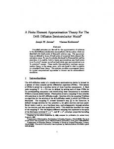
where in the last step we have used the second interpolation estimate in (31) with s = 23 + ǫ < 1 + t. Note also that in the first step the fractional derivative in the norm in H ǫ (∂K) would scale as hǫK , but we need to introduce a length scale ℓ independent of the element size to bound the whole H ǫ (∂K)-norm. Combining the previous results, we easily get the desired error estimate. Remark 3.2. Assumption 1 is known to hold for k ≥ 4 in dimension 2. In this case, we can take Gh as the finite element space obtained for the Argyris triangle. For k ≥ 2, Gh can be constructed by using the Bogner-Fox-Schmidt triangle; in order to do this, the triangulation Th should admit a coarser mesh of macroelements. Under the same kind of restriction over the mesh topology, the discrete space recently introduced in [31], based on a Powell–Sabin interpolant (see Figure 1 right), makes true Assumption 1 for k ≥ 1, both in two and three dimensions (see also [12, 6, 26]). Furthermore, we have observed from numerical experiments that a mesh with the crossed-box typology (see Figure 1 left) also satisfies this assumption. In a numerical code, it implies to perform a pre-processing of the original mesh. Given an original triangular mesh, the Powell-Sabin mesh is obtained by introducing additional nodes on the mid-points of the edges and the element barycentes, and re-connecting the nodes properly. On the other hand, crossed-box meshes are obtained from a quadrilateral mesh by placing a node on its center, and creating four triangles; in fact, the additional node can be condensed. These are the two typologies of meshes considered in Section 4. Other typologies may fail to converge for singular solutions not belonging to H 1 (Ω). Three-dimensional extensions of these elements have already been designed and implemented, showing excellent results for singular solutions.

Figure 1: Crossed-box (left) and Powell-Sabin (right) macro-element typologies.

14

Remark 3.3. When Assumption 1 is satisfied, the previous result is very strong, in the sense that we have not only proved convergence towards the good solution, but an (almost) optimal order of convergence, even for nonsmooth solutions. We can also weaken the approximability assumption over Gh , and in the limit case lim inf kφ − φh kH s (Ω) = 0,

h→0 φh ∈Gh

s ≤ 1 + r,

we would get strong convergence towards the solution without order. Alternatively, instead of considering the decomposition of u, an interpolation result lim inf ℓr−1 ku − wh kH r (Ω) + k∇ × (u − wh )k = 0, h→0 wh ∈Vh

for Vh would also lead to convergence towards the good solution, without the need to introduce Gh .

4 Numerical experiments 4.1 Stabilized curl formulation In order to check, using numerical experimentation, that the nodal-based finite element approximation proposed in this article converges to both smooth and nonsmooth physical solutions, we take the datum f such that the solution of (3) in polar coordinates (r, θ) is: 2n 2nθ 3 (32) u = ∇ r sin 3 in the nonconvex domain Ω ≡ [−1, 1]2 \ [0, 1]2 , with one re-entrant corner. We have 2n that u ∈ H 3 −ǫ (Ω), for any ǫ > 0. Since for n = 1 we have that u 6∈ H 1 (Ω), by virtue of Corollary 3.1, curl-div based finite element approximations converge to spurious solutions. On the other hand, as proved in Theorem 3.1, the solution of formulation (15) must converge to the physical solution (32) by using h-refinement and appropriate meshes. In order to observe this, we have considered a family of structured triangular meshes obtained by a partition of the domain into squares and a subsequent division of the squares in the crossed-box fashion (see Figure 1). The number of divisions in every direction has been set to 2i with i = 3, 4, 5, 6; the characteristic mesh size h is 2−i and the number of triangular elements 2i+1 . In Figure 2(a), we show the numerical errors eu = uh − u and ep = ph − p for different norms as h → 0. The convergence rate at every refinement level and numerical values of the error have been provided in Table 1. From these results, it is clear that the method we propose herein is capable to approximate numerically nonsmooth solutions, as Theorem 3.1 says. In fact, the order of convergence of the method is surprisingly high when compared to those for the weighted regularization in [10] and the discontinuous Galerkin technique in [21] (for the same test problem). Now, in order to stress the importance of the hk∇ · uh k stability, we have switched off the term h2K ∇ · uh , ∇ · vh from the formulation (15). In the previous stability analysis, this term is crucial for recovering L2 (Ω)-control of uh . We perform the same convergence test as above and show the plots in Figure 2(b). As expected, convergence is not attained for the quantity keu k. So, the introduction of this term is motivated by both theoretical and numerical observations. 15

0.5

−0.5 −1

−1

−1.5 −2

−1.5 −2 −2.5 −3

−2.5 −3 −1.8

−3.5 −1.6

−1.4

−1.2 −1 log(h)

−0.8

−4 −1.8

−0.6

(a) n = 1

−1.6

−1.4

−1.2 −1 log(h)

−0.8

−0.6

(b) n = 1 without div-div term −1

−0.5

u curl(u) p grad(p) slope 1 slope 2

−1.5 −2


−2 log(|| error ||)

−1

log(|| error ||)


−0.5

log(|| error ||)

0

log(|| error ||)

0


−2.5

−3

−4

−3

−5 −3.5 −4 −1.8

−1.6

−1.4

−1.2 −1 log(h)

−0.8

−6 −1.8

−0.6

(c) n = 2

−1.6

−1.4

−1.2 −1 log(h)

−0.8

−0.6

(d) n = 4

Figure 2: Error plots for different quantities in L2 (Ω) norm for Formulation (15) and the problem with analytical solution (32), with different values of n. Plot (b) corresponds to (15) without the stabilization term su (uh , vh ). Going back to the full formulation (15), we perform the same convergence analysis with n = 2 and n = 4 in (32). In the case n = 2, the solution uh belongs to 4 H 3 −ǫ (Ω) ⊂ H 1 (Ω). Then, both curl-div and curl formulations are able to capture the solution. In any case, the smoothness of the solution does not allow us to obtain theoretically optimal convergence for first order approximation of both uh and ph , since u 6∈ H 2 (Ω). The convergence plot and convergence rates at every level of refinement can be found in Figure 2(c) and Table 2, respectively. The method exhibits some super8 convergence. Finally, for n = 4 the solution u belongs to H 3 −ǫ (Ω) and the optimal error estimate should apply. We can see that this is in fact the case for both u and p in the continuous norm |||eu , ep ||| in Figure 2(d) and Table 1. Again, the method exhibits super-convergence. Finally, we solve the singular problem (with n = 1) with a Powell-Sabin mesh. As expected, the method shows a very similar convergence order as the one obtained for crossed-box meshes. The numerical errors and slopes with respect to h are shown in table 3.

16

Table 1: Experimental errors for Method (15) for uh and rate of convergence (in brackets). Piecewise linear finite elements for both uh and p. h

keu k

n=1 k∇ × eu k

keu k

n=2 k∇ × eu k

keu k

n=4 k∇ × eu k

2−3

2.67e-1 (-)

3.92e-1 (-)

6.75e-2 (-)

9.96e-2 (-)

7.31e-3 (-)

2.66e-2 (-)

2−4

1.51e-1 (0.82)

2.03e-1 (0.95)

2.49e-2 (1.44)

3.20e-2 (1.64)

1.93e-3 (1.92)

3.44e-3 (2.95)

2−5

8.11e-2 (0.90)

9.22e-2 (1.14)

8.68e-3 (1.52)

9.08e-3 (1.82)

4.89e-4 (1.98)

4.34e-4 (2.99)

2−6

4.52e-2 (0.84)

3.98e-2 (1.21)

3.12e-3 (1.48)

2.44e-3 (1.89)

1.22e-4 (2.00)

5.43e-5 (3.00)

Table 2: Experimental errors for Method (15) for ph and rate of convergence (in brackets). Piecewise linear finite elements for both uh and p. n=1

n=2

n=4

h

kep k

k∇ep k

kep k

k∇ep k

kep k

k∇ep k

2−3

1.56e-1 (-)

1.05e+0 (-)

3.72e-2 (-)

2.68e-1 (-)

8.69e-4 (-)

1.14e-2 (-)

2−4

8.70e-2 (0.83)

8.75e-1 (0.27)

1.30e-2 (1.51)

1.39e-1 (0.95)

1.01e-4 (3.10)

2.10e-3 (2.44)

2−5

4.09e-2 (1.09)

6.29e-1 (0.48)

3.85e-3 (1.76)

6.27e-2 (1.15)

1.09e-5 (3.22)

3.56e-4 (2.56)

2−6

1.76e-2 (1.22)

4.19e-1 (0.59)

1.04e-3 (1.89)

2.63e-2 (1.25)

1.10e-6 (3.30)

5.88e-5 (2.60)

Table 3: Experimental errors for Method (15) for uh and rate of convergence (in brackets) for the test problem with n = 1 and Powell-Sabin triangle meshes. Piecewise linear finite elements for both uh and p. h

keu k

n=1 k∇ × eu k

2−3

2.13e-1e-1 (-)

2.99e-1 (-)

2−4

1.13e-1 (0.91)

1.40e-1 (1.10)

2−5

5.98e-2 (0.92)

5.99e-2 (1.22)

2−6

3.34e-2 (0.84)

2.48e-2 (1.27)

17

4.2 Stabilized curl-div formulation Following the same idea as at the continuous level, in which we went from (3) to (4) passing regularity from p to u, we can pass from (15) to a curl-div stabilized finite element formulation. Proceeding this way, we get the discrete problem: find uh ∈ Vh and ph ∈ Qh solution of a(uh , vh ) + b(vh , ph ) + (cu λ∇ · uh , ∇ · vh ) = (f , vh ) , X Z h2 K ∇ph · ∇qh dx = 0, −b(uh , qh ) + K λ

∀vh ∈ Vh ,

(33a)

∀qh ∈ Qh .

(33b)

K∈Th

Again, this method is a residual-based finite element method, in which the stabilization parameter has been chosen to be cu λ. The second term in the right-hand side h2 comes from the penalty term in (9) but taking λK as penalty coefficient. The numerical analysis of this method uses similar arguments to the ones for (15). Since we have control over both the curl and the divergence of uh , and the control hk∇ph k only leads to L2 (Ω) stability for ph , this problem is well-posed for the curl-div norm, for which there is no approximability property. Thus, this formulation is not able to deal with the singular solution (32) with n = 1; we show this in Figure 3(a). However, as expected, the method converges for n = 2 and n = 4 to the good solution, since u ∈ H 1 (Ω). We show the error plots in Figures 3(b) and 3(c). Let us point out that in the curl-div formulation there is no control over ∇ph , and so, no convergence can be expected for it (see Figure 3(b)).

5 Conclusions The finite element formulation proposed in this paper to approximate Maxwell’s problem has been shown to allow one to use continuous Lagrangian interpolations for the unknown, yielding stable and convergent approximations to any solution of the continuous problem, including singular solutions. Convergence to smooth solutions is reached with optimal order. The essential point to converge to singular solutions is to avoid the spurious control on the L2 (Ω)-norm of the divergence of the unknown, typical of penalized or curl-div formulations. Instead of avoiding this by using weighted L2 (Ω)-inner products, we resort to the introduction of a Lagrange multiplier to enforce the zero divergence restriction. However, to ensure stability of this in the appropriate functional setting, a novel augmented formulation has been introduced, which consists of adding a Laplacian of the multiplier in the zero divergence restriction. Since the multiplier is zero in the continuous problem, consistency remains unaltered. The final ingredient is to use a stabilized formulation at the discrete level, in our case consisting only in adding a leastsquare form of the zero divergence condition. The stabilizing term is multiplied by the square of the mesh size, so that it mimics stability of the divergence of the unknown in H −1 (Ω), not in L2 (Ω), as curl-div formulations wrongly do. This new term is also responsible for obtaining stability in the L2 (Ω) part of the whole H(curl; Ω) norm of the unknown. Finally, in order to have approximability, particular mesh typologies must be used for singular solutions, at least for linear Lagrangian elements, that can easily be generated post-processing any original triangular or quadrilateral mesh. A classical numerical test has been used to check the theoretical predictions. Notably, very good convergence has been observed in the case when the solution is singular, as compared to other formulations that can be found in the literature. 18

1

1.5


log(|| error ||)

0.5 0


0 log(|| error ||)

1

−0.5 −1 −1.5

−1

−2

−3

−2 −2.5 −1.8

−1.6

−1.4

−1.2 −1 log(h)

−0.8

−4 −1.8

−0.6

−1.6

(a) n = 1

−1.2 −1 log(h)

−0.8

−0.6

(b) n = 2 0


−1 log(|| error ||)

−1.4

−2

−3

−4

−5 −1.8

−1.6

−1.4

−1.2 −1 log(h)

−0.8

−0.6

(c) n = 4

Figure 3: Error plots for different quantities in L2 (Ω) norm for Formulation (33) and the problem with analytical solution (32), with different values of n. The practical interest of our approach is clear. Even if tailored approximations for Maxwell’s problem may be afforded at a reasonable computational cost when it is an isolated problem, it is obvious that a classical Lagrangian type approximation greatly simplifies its implementation in situations where this problem is coupled to others, as in MHD. On the other hand, our approach may be viewed as an alternative to the use of the so called compatible discretization, satisfying the appropriate inf-sup conditions. In simple model problems, such as Stokes’, Maxwell’s and Darcy’s, our formulation allows us to use the same interpolation for the unknowns in all cases, instead of one compatible for each case.

References [1] C. Amrouche, C. Bernardi, M. Dauge, and V. Girault. Vector potentials in threedimensional non-smooth domains. Mathematical Methods in the Applied Sciences, 21(9):823–864, 1998. [2] F. Assous, P. Ciarlet Jr., S. Labrunie, and J. Segré. Numerical solution to the timedependent Maxwell equations in axisymmetric singular domains: the singular complement method. Journal of Computational Physics, 191:147–176, 2003.

19

[3] S. Badia and R. Codina. Unified stabilized finite element formulations for the Stokes and the Darcy problems. SIAM Journal on Numerical Analysis, 47(3):1977–2000, 2009. [4] S.C. Brenner and L.R. Scott. The Mathematical Theory of Finite Element Methods. Springer–Verlag, 1994. [5] F. Brezzi and M. Fortin. Mixed and Hybrid Finite Element Methods. Springer Verlag, 1991. [6] A. Buffa, P. Ciarlet Jr., and E. Jamelot. Solving electromagnetic eigenvalue problems in polyhedral domains with nodal finite elements. Numerische Mathematik, 113(4):497–518, 2009. [7] R. Codina. A stabilized finite element method for generalized stationary incompressible flows. Computer Methods in Applied Mechanics and Engineering, 190:2681–2706, 2001. [8] R. Codina. Analysis of a stabilized finite element approximation of the Oseen equations using orthogonal subscales. Applied Numerical Mathematics, 58:264– 283, 2008. [9] R. Codina, J. Principe, O. Guasch, and S. Badia. Time dependent subscales in the stabilized finite element approximation of incompressible flow problems. Computer Methods in Applied Mechanics and Engineering, 196:2413–2430, 2007. [10] M. Costabel. A coercive bilinear form for Maxwell’s equations. Journal of Mathematical Analysis and Applications, 157(2):527–541, 1991. [11] M. Costabel and M. Dauge. Singularities of electromagnetic fields in polyhedral domains. Archives for Rational Mechanics and Analysis, 151(3):221–276, 2000. [12] M. Costabel and M. Dauge. Weighted regularization of Maxwell equations in polyhedral domains. Numerische Mathematik, 93(2):239–277, 2002. [13] H.Y. Duan, F. Jia, P. Lin, and R.C.E. Tan. The local L2 projected C 0 finite element method for Maxwell problem. SIAM Journal on Numerical Analysis, 47(2):1274– 1303, 2009. [14] A. Ern and J.L. Guermond. Theory and Practice of Finite Elements. Springer– Verlag, 2004. [15] V. Girault and P.A. Raviart. Finite Element Methods for Navier-Stokes Equations. Springer–Verlag, 1986. [16] M. Grote, A. Schneebeli, and D. Schötzau. Interior penalty discontinuous galerkin method for Maxwell’s equations: energy norm error estimates. Journal of Computational and Applied Mathematics, 204(375–386), 2007. [17] M.J. Grote, A. Schneebeli, and D. Schötzau. Interior penalty discontinuous galerkin method for Maxwell’s equations: optimal L2 -norm error estimates. IMA Journal of Numerical Analysis, 28:440–468, 2008. [18] C. Hazard. Numerical simulation of corner singularities: a paradox in Maxwelllike problems. Comptes Rendus-Mécanique, 330(1):57–68, 2002. 20

[19] C. Hazard and M. Lenoir. On the solution of time-harmonic scattering problems for Maxwell’s equations. SIAM Journal on Mathematical Analysis, 6(1597– 1630):1996, 27. [20] R. Hiptmair. Finite elements in computational electromagnetism. Acta Numerica, 11(237–339), 2003. [21] P. Houston, I. Perugia, and D. Schötzau. Mixed discontinuous Galerkin approximation of the Maxwell operator. SIAM Journal on Numerical Analysis, 42(1):434–459, 2005. [22] T.J.R. Hughes. Multiscale phenomena: Green’s function, the Dirichlet-toNeumann formulation, subgrid scale models, bubbles and the origins of stabilized formulations. Computer Methods in Applied Mechanics and Engineering, 127:387–401, 1995. [23] B. Jiang, J. Wu, and L.A. Povinelli. The origin of spurious solutions in computational electromagnetics. Journal of Computational Physics, 125(1):104–123, 1996. [24] J. Jin. The Finite Element Method in Electromagnetics. Wiley, 1993. [25] P. Ciarlet Jr. Augmented formulations for solving Maxwell equations. Computer Methods in Applied Mechanics and Engineering, 194(559–586), 2005. [26] P. Ciarlet Jr. and G. Hechme. Mixed, augmented variational formulations for Maxwell’s equations: numerical analysis via the macroelement technique. Submitted, 2009. [27] P. Monk. Finite Element Methods for Maxwell’s Equations. Oxford University Press, 2003. [28] S. Nicaise. Edge elements on anisotropic meshes and approximation of the Maxwell equations. SIAM Journal on Numerical Analysis, 39(3):784–816, 2001. [29] I. Perugia, D. Schötzau, and P. Monk. Stabilized interior penalty methods for the time-harmonic maxwell equations. Computer Methods in Applied Mechanics and Engineering, 191:4675–4697, 2002. [30] D. Schötzau. Mixed finite element methods for stationary incompressible magneto-hydrodynamics. Numerische Mathematik, 96:771–800, 2004. [31] T. Sorokina and A.J. Worsey. A multivariate Powell–Sabin interpolant. Advances in Computational Mathematics, 29(1):71–89, 2008.

21