OCEANOLOGICA ACTA ⋅ VOL. 24 – No. 5
A non-linear software sensor to monitor the internal nitrogen quota of phytoplanktonic cells Olivier BERNARDa*, Antoine SCIANDRAb, Gauthier SALLETc a
Inria, Comore, BP 93, 06902 Sophia-Antipolis cedex, France LOV, Station zoologique, BP 28, 06230 Villefranche-sur-Mer, France c Inria-Lorraîne, ISGMP, Île de Saulcy, 57045 Metz cedex 01, France b
Abstract − New techniques – called software sensors – issued from the non-linear automatic control field and initially developed for non-linear chemical systems have been applied to a continuous culture of phytoplankton. A software sensor (or ‘observer’) combines an analytical differential equation based model and partial measurements of the system in order to estimate the non-measured state variables. It filters data and estimates the actual state of living systems, models of which are often rough approximations. The efficiency of this approach is illustrated with a nitrate-limited chemostat experiment with the chlorophyceae Dunaliella tertiolecta performed in a computer controlled fluctuating environment. © 2001 Ifremer/CNRS/IRD/Éditions scientifiques et médicales Elsevier SAS Résumé − Un capteur logiciel non linéaire pour estimer le quota interne en azote de cellules phytoplanctoniques. Des observateurs issus de la science du contrôle et initialement développés pour des systèmes chimiques non linéaires ont été appliqués à des cultures continues de phytoplancton. Un observateur, ou « capteur logiciel », combine un modèle à base d’équations différentielles et des mesures parcellaires sur le système afin d’estimer les variables internes non mesurées. Cet outil filtre les mesures et estime l’état réel des systèmes vivants dont les modèles sont souvent très approximatifs. L’efficacité de cette approche est illustrée sur des expériences en chémostat avec la chlorophyceae Dunaliella tertiolecta carencée en azote dans un environnement fluctuant piloté par ordinateurs. © 2001 Ifremer/CNRS/IRD/Éditions scientifiques et médicales Elsevier SAS Droop model / non-linear systems / observers / phytoplankton modèle de Droop / systèmes non linéaires / observateurs / phytoplancton
1. INTRODUCTION
to reduce the effects of noise of measurements as well as to estimate variables which are not measured. These tools originated from control science, and were initially developed for linear systems (Luenberger, 1966), and have been more recently extended to non-linear chemical systems. They are based on mathematical model outputs constantly modified by a process of trajectory adjustments driven by the partial measurements obtained from the system (see figure 1). If the model fulfils the so-called ‘observability’ properties (see appendix A), the software sensor provides real-time estimates of the key process variables from the available on-line measurements. The point of this theoretical device lies in the juxtaposition of the two types of information available on the system: its theoretical behaviour, supported by the model, and its observed behaviour, represented by the on-line measurements. Their success
The key role played by phytoplankton in the oceanic carbon cycle has enhanced the studies aiming to improve the understanding and the modelling of the phytoplanktonic growth. It is therefore important to have sensors that can precisely monitor the internal state of the phytoplanktonic cells during experiments. However, there is a lack of reliable sensors able to provide high frequency estimations of biological signals such as biomasses or related physiological variables. We show here that it is possible to overcome this by employing software sensors, i.e. algorithms that are used *Correspondence and reprints: fax: +33 492 387 858. E-mail address:
[email protected] (O. Bernard).
© 2001 Ifremer/CNRS/IRD/Éditions scientifiques et médicales Elsevier SAS. Tous droits réservés S0399178401011550/FLA
435
O. Bernard et al. / Oceanologica Acta 24 (2001) 435–442
Figure 1. Synoptic diagram of a software sensor. It combines the theoretical knowledge of a system through a mathematical model, and the practical knowledge of its actual functioning through measurements. If the inputs acting on the system are known (and provided that theoretical conditions are fulfilled (appendix A)), and if, moreover, the model is a sufficient approximation of the real system, then the software sensor estimates the whole state of the system.
term for nutrient uptake, allowed Burmaster (1979) to compose an ordinary differential equation based model for phytoplanktonic cells (biomass N) growing in a chemostat under a single nutrient limitation:
relies on the fact that stochastic uncertainty on parameters gives rise to a noise on the measured signal which is then filtered by the software sensor. In this paper, we propose to design a non-linear software sensor for a culture in chemostat of the green algae Dunaliella tertiolecta. We first present the Droop model describing the growth of phytoplanktonic cells under nutrient limitations in continuous culture (chemostat). We then define a class of models broader than the Droop model that finds numerous applications in ecology and oceanography. These models fulfil the appropriate conditions that guarantee the exponential convergence of the non-linear observers. We also present the observer for these models and derive a high gain observer based on the Droop model for the monitoring of phytoplankton. After a review of the materials and methods used, we apply the software sensor to real experiments, and we draw conclusions on the validity and on the efficiency of the software sensor.
共 RD 兲
冦
S~共 t 兲 = D 关 Sin − S共 t 兲 兴 − qm
冉
冊
S共 t 兲 N共 t 兲 kS + S共 t 兲
kQ N共 t 兲 − DN共 t 兲 Q共 t 兲 S共 t 兲 Q ~共 t 兲 = qm − µfl 共 Q共 t 兲 − kQ 兲 kS + S共 t 兲
N~共 t 兲 = µfl 1 −
(1)
The parameters qm and kS represent respectively the maximum uptake rate and the half-saturation constant for the substrate. kQ is the minimum internal quota allowing growth and µfl is the hypothetical growth rate obtained for an infinite quota. The dilution rate D is the quotient of the medium inflow rate over the chemostat volume. The substrate concentration in the renewal medium is denoted Sin. The model parameters have been calibrated using chemostat steady state conditions and batch experiments (table I).
2. THE DROOP MODEL The modelling of phytoplankton growth under substrate limitation has been under development during the past 30 years. In contrast to bacteria whose growth can be represented by the simple Monod model (Monod, 1942), phytoplankton shows a strong uncoupling between nutrient uptake and growth (Cunningham and Maas, 1978; Sciandra, 1991). A modelling of this phenomenon has been proposed by Droop (1968) and Caperon and Meyer (1972) who represented growth as dependent not on external substrate (of concentration S), but on an internal quota (Q) defined as the quantity of nutrient per biomass unit. This empirical law, combined with Dugdale’s (1967)
Table I. Parameters of the Droop model for Dunaliella tertiolecta 2pt grown at 20 °C. With v共 t 兲 = 35 1 + 0.3 sin . SD, StanT dard deviation.
共
关
Parameters
qm kS µfl kQ D T Sin
436
Units
Values –3
–1
µmol·µm ·d µmol·L–1 d–1 µmol·µm–3·d–1 d–1 d µmol·L–1
兲兴
SD –9
8.38 10 0.12 1.85 1.5 10–9 0.96 1.0 v(t)
1.20 10–9 0.10 0.30 0.2 10–9 0.02 0.0 1.0
O. Bernard et al. / Oceanologica Acta 24 (2001) 435–442
of system has been called the Strictly Linked Lower Hessenberg (SL2H) systems. It is defined as follows:
Let us denote y the available on-line measurement. Here, y is the biomass, estimated by the measurements of total biovolume (see section 4). We will consider experiments where the concentration of nitrate in the renewal medium Sin, varies in the following manner: Sin = si(1 + u), u being the input forcing the system (u > –1), and si the nitrate concentration in the influent without input (u = 0).
Definition 1 (SL2H systems). A system (Σ) is said to be SL2H if it satisfies the following conditions for any x and any u (belonging to the considered domain): – 1. for any indexes (i, j) such that j > (i + 1): ⭸Fi x, u 兲 = 0 ⭸xj 共 ⭸Fi – 2. for any index i: x, u 兲 7 0 ⭸xi + 1 共 – 3. h(x) = h(x1), with dh 共 x1 兲 7 0. dx1
Let us do the following change of variable: qm N ; x2 = Q ; x3 = S si kQ si kS qm • a1 = ; a2 = µfl ; a3 = si kQ
• x1 =
3.2. Example of SL2H systems
The model reduces now to: 共 RD 兲
再
x˙ = f共 x 兲 + ug共 x 兲 y = h共 x1 兲
t first, models describing the growth of a stage structured population are usually represented by Leslie-type (Caswell, 1989; Sciandra, 1986) systems which are SL2H:
(2)
with:
x=
冉冊
x1 x2 , f共 x 兲 = x3
g共 x 兲 =
冉冊
冢
共
兲
a2 1 − 1 x1 − Dx1 x2 x3 a3 − a2共 x2 − 1 兲 a1 + x3 x1 x3 D共 1 − x3 兲 − a1 + x3
冣
再
(3)
for i ∈ 兵 1, ..., n − 1 其
(5)
In these models x1 represents adults and xn the youngest stage (often eggs). The function Fn describes the socalled recruitment process, i.e. eggs laying from the other ⭸Fi stages. The term corresponds to the transfer rate ⭸xi + 1 from stage i to stage i+1, which is never zero.
0 0 , h共 x1 兲 = x1 D
A second broad class of SL2H systems is composed by models describing trophic chains (Rosenzweig, 1973; Hastings and Powell, 1991). These models represent the dynamics of an ecosystem from nutrient (x1), phytoplankton (x2), etc. to higher levels such as fishes (xn). They can be written:
3. OBSERVABILITY AND HIGH GAIN OBSERVERS FOR THE DROOP MODEL 3.1. Definition
再
In order to explain in a general framework how to build a software sensor, we consider the general differential system (Σ), that represents the evolution of the internal state x (vector for all the variables):
再
x˙i = Fi共 xi, xi + 1 兲 x˙n = Fn共 x1, x2, ..., xn 兲
x˙1 = F1共 x1, x2 兲 x˙i = Fi共 xi − 1, xi, xi + 1 兲 for i ∈ 兵 2, ..., n − 1 其 x˙n = Fn共 xn − 1, xn 兲
(6)
(4)
The interactions between variables are expressed by functional responses which are generally monotonous functions of the predator, so that these models are SL2H.
We will show that numerous biological models have a specific structure which guarantees the observability (see the definition in appendix A) conditions and for which the construction of an observer is straightforward. This class
Another important class of systems in biology are the loop-structured systems with monotonous interactions (Goodwin, 1965; Levine, 1985; Bernard and Gouzé, 1995), which are encountered when describing gene regulation, enzymatic chains, biosynthetic pathway, etc.
共R兲
x˙共 t 兲 = F共 x共 t 兲, u共 t 兲 兲 = f共 x 兲 + ug共 x 兲 y共 t 兲 = h共 x共 t 兲 兲 x共 0 兲 = x0
437
O. Bernard et al. / Oceanologica Acta 24 (2001) 435–442
From Property 1 (cf. appendix A), a high gain observer can be derived for the Droop model. The delicate point consists in proving that the required theoretical hypothesis (H1) holds for the Droop model (see Bernard et al., 1999, for details).
These systems constitutes also a peculiar case of SL2H systems (indices are denoted modulo n):
兵 x˙i = Fi共 xi, xi + 1 兲 for i ∈ 兵 1, ..., n 其
(7)
⭸Fi 7 0 for i ∈ 兵 1, ..., n 其 . The Droop model ⭸xi + 1 belongs to this class of models.
with
The differential system corresponding to the software sensor for the Droop model is given by equation (8) with:
In the next section, we see that SL2H systems verify (under additional reasonable hypotheses) conditions ensuring the exponential convergence of the high gain observers (Deza et al., 1992; Gauthier et al., 1992).
G共 xˆ 兲 =
3.3. Observers for SL2H systems As it is detailed in appendix B, under some additional technical hypotheses, a so-called high gain observer can be designed for SL2H systems. It provides an estimate (denoted xˆ 兲 of the internal state vector x. It is mainly a copy of the model plus a correction term based on the comparison between the predicted measures 共 h共 xˆ1 兲 兲 and the actual ones (y). The predictions of the observer 共 xˆ 兲 converge toward the real state x. The differential system corresponding to the software sensor is then the following: | 兲 兵 xˆ = f共 xˆ 兲 + ug共 xˆ 兲 + G共 xˆ 兲共 y − h共 xˆ1 兲 兲 共R
B|31 =
3h
关 共
2
兲 兴
册 册
xˆ2 2 xˆ2 1 − 1 − D xˆ2 + 3h xˆ1 a2 a2xˆ1 2
xˆ2共 a1 + xˆ3 兲 a1 a2 a3xˆ1 2
3hB|31 + 3h B|32 + h
3
2
冣
冋
冉
冊
2 a3xˆ3 2 1 + 2a2 + xˆ2 2a2 − 3D − D − a1 a3xˆ1 a1 + xˆ3 a2 a3xˆ3 1 − D + 4a2 − 4D xˆ2 2 a1 + xˆ3 a2
冉
xˆ2共 a1 + xˆ3 兲 a1 a2 a3xˆ1
冋
共
兲
2
B|32 =
(8)
xˆ2共 2D − 3a2 兲 + 4a2 + 2
a3xˆ3 a1 + xˆ3
冊册 册
4. MATERIALS AND METHODS 4.1. The culture system The basic culture system has been described by Bermard et al. (1996). The chemostat consisted of a 1.8-L doublejacketed glass vessel thermostated at 20 °C within 0.05 °C (see figure 2). The seawater was filtered through 0.2-µm Millipore filters and autoclaved for 1 h at 115 °C. After cooling, sterile f/2 medium without nitrate (NO3) or silicate was added. A sterile concentrate of NO3 was mixed into the enrichment medium before supplying the chemostat. Magnetic stirrers ensured homogeneous media. Air, passed through a 0.1-mm Whatman filter and activated charcoal, was bubbled with a 9-L·h–1 flow rate into the chemostats. The turbulent energy resulting from bubbling and stirring was sufficient to prevent the cells from sticking to the vessel walls, at least for 1 month, and to ensure the homogeneity of the culture. In the chemostat mode, the liquid volumes were kept constant by continuously removing medium from the surface of the culture. The cultures were grown using a flood-light
3.4. Observability and observer for the Droop model We first show that the Droop model is a SL2H model, as defined in Definition 1. Indeed, we have: x1 ⭸F1 = a2 2 > 0, ⭸x2 x2 ⭸F2 a1 = a3 2 > 0 and moreover: ⭸x3 共 a1 + x3 兲 and
冋 冋
where:
The term G共 xˆ 兲 is a matrix, called the gain matrix, which depends on the estimate xˆ. This gain matrix also contains a parameter allowing the tuning of the convergence rate of the software sensor. The main point to design the observer is the computation of this gain matrix (see appendix B for the general case). The expression of G共 xˆ 兲 for the Droop model is detailed in the next paragraph.
⭸F1 =0 ⭸x2
冢
3h
⭸h = 1. ⭸x1 438
O. Bernard et al. / Oceanologica Acta 24 (2001) 435–442
automatic sampler (Model 3000), is monitored by a computer using particle distribution analysis software (PDAS). Before counting, dilution of concentrated phytoplankton cultures is necessary. This is routinely performed by an automatic system constituted by peristaltic pumps (GILSON), solenoid valves, and a syringe commanded by another computer.
projector provided with two 150-W metal halide lamps (Osram, HQI) and one anti-UV glass-screen. The possible small remainder of UV energy was definitely cut off by the 1-cm thick Plexiglas covers of the growth chamber. Before the beginning of experiment, algae were starved for 3 d by reducing the enrichment level from si = 35 µmol·L–1 (corresponding to biomass steady state) to 8 µmol·L–1.
To estimate the internal quota, measures of particulate nitrogen were performed, with a CHN analyser (LECO 900) after filtration through Whatman GFF filters. These off-line measures are used to estimate the total quantity of particulate nitrogen NT in the chemostat. The internal quota Q is then estimated as follows: Q = NT/N.
4.2. Nutrient analysis To ensure the automation of a Technicon Auto-analyser, a set of pumps and electric valves are controlled by a PC computer. Sampling, filtration through Gelman A/E filters, and output signal acquisition from both colorimeters (NO2 and NO3) are programmed in time with specified intervals. The system standardizes itself by calculating the respective gains of the colorimeters and the cadmiumcopper column efficiency (Bernard et al., 1996).
4.4. Control of nutrient supply Peristaltic pumps (GILSON) provide axenic enrichment medium into the chemostat after mixing the f/2 medium without NO3 and a concentrated solution of NaNO3. For this, a dedicated computer controlled system drives a double solenoid valve allowing the concentrated solution of NaNO3 to be replaced with seawater without NO3. This manner of actuating the pump is used to give to the renewal medium concentration any dynamic pattern by computing every 5 min the proportion of time seawater replaces the concentrated NaNO3 solution (Bernard et al., 1996).
4.3. Cell counting Size spectra and cell concentrations are obtained by the particle counter HIAC/ROYCO PACIFIC. The system, constituted by an optical sensor (Laser sensor HRLD400), high-speed digital counter (Model 9064) and an
Figure 2. Synoptic diagram of the culturing system. The three tanks for the nutrient supply system are: 1: sterile f/2 medium without nitrate, 2: sterile seawater with high nitrate concentration, 3: sterile seawater without nitrate.
439
O. Bernard et al. / Oceanologica Acta 24 (2001) 435–442
5. RESULTS The high gain software sensor (equation (8)) was tested on experiments with the autotrophic chlorophyceae Dunaliella tertiolecta grown under nitrate limitation in a fluctuating chemostat environment controlled by computers. From the on-line biomass measurements, the software sensor computes the nitrate concentration in the medium and the internal quota of the phytoplankton. A periodic pattern of the influent nitrate concentration has been applied in order to reproduce certain marine hydrodynamical conditions. These experiments were used to test the software sensor when a dynamical forcing of the system is maintained. In spite of its intensive use, the validation works of the Droop model have only been done at equilibrium (Goldman and Peavey, 1979; Sciandra and Ramani, 1994). This model has been established in classical chemostat conditions, i.e. for the equilibria obtained in different stable nutrient environments. The main question of this work is to know whether the software sensor based on the Droop model can accurately estimate the variables for a nutrient fluctuating environment. The software sensor first acts as a filter for biomass (figure 3). Indeed, it smoothes the noisy signal of the biomass measurements (estimated with total biovolume). Its main function is nevertheless to compute unmeasured variables. It can be seen that the software sensor substrate estimations are very close to the direct measurements which currently requires sophisticated and delicate devices under the supervision of a microcomputer. In this case, it can replace or back up fastidious measurements. In regard to the internal quota, it can provide an estimation, at least for established conditions (after day 2).
Figure 3. Comparison between measurements (•) and software sensors predictions (––) for the Droop model. A. Biomass described by total biovolume of algae. B. Internal quota. C. Nitrate concentration. The gain of the software sensor is θ = 1.
One could argue that the transient biased observer estimation at the very beginning of the experiment can be due to the normal period necessary for the convergence. In particular, the high gain observer is known to give rise in certain situations to rapid excursions that can lead to transient predictions far from the real values of the state variables (picking phenomenon). To avoid this artefact, a relatively small gain has been chosen (θ = 1) and the observer has been initiated at the exact initial experimental conditions. This should, if the model were exact, have avoided the transient convergence period of the observer.
out two modelling defects. First, the internal quota predictions are overestimated during the first 2 d of experiment. This lack of observer convergence indicates a bias in growth rate modelling: the rapid evolution in biovolume at the beginning of the experiment is above the maximum expected growth rate µmax. This theoretical threshold can be calculated when considering algae growing in an unlimited environment. The hypothesis S