Also, the seasonal adjustment method should have the recovery property, as well .... chose the Box-Jenkins Airline model for our model class in order to fix our ...
RESEARCH REPORT SERIES (Statistics #2008-1)
A Nonlinear Algorithm for Seasonal Adjustment in Multiplicative Component Decompositions Tucker McElroy
Statistical Research Division U.S. Census Bureau Washington, DC 20233
Report Issued: February 21, 2008 Disclaimer: This paper is released to inform interested parties of research and to encourage discussion. The views expressed are those of the author and not necessarily those of the U.S. Census Bureau.
A Nonlinear Algorithm for Seasonal Adjustment in Multiplicative Component Decompositions Tucker McElroy U.S. Census Bureau
Abstract We propose a new model-based, nonlinear method for seasonally adjusting time series in a multiplicative components model. The method seeks to reduce the bias inherent in linear modelbased approaches, while at the same time preserving the flexibility of parametric methods. We discuss the problem of bias and the concept of recovery, and demonstrate the favorable properties of the proposed algorithm on several synthetic series.
Keywords. Nonstationary time series, Seasonality, Trends Disclaimer This report is released to inform interested parties of research and to encourage discussion. The views expressed on statistical issues are those of the author and not necessarily those of the U.S. Census Bureau.
1
Introduction
Many economic time series exhibiting seasonality are naturally explained via a multiplicative components decomposition; a very common three-component decomposition is given by yτ = sτ · tτ · iτ
(1)
where y is the observed data (with outliers and other regression effects removed), s is the seasonal component, t is the trend component, and i is the irregular. We index time with the variable τ = 1, 2, · · · , N . This description of the data is justified empirically by the observation that the variability in seasonal fluctuations seems roughly proportional to the trend level for many economic series – see Findley, Monsell, Bell, Otto, and Chen (1998) and the references therein for additional discussion. The goal of seasonal adjustment is estimation of sτ for each τ ; we then obtain the seasonally adjusted data by dividing the seasonal estimate into yτ . In the vast literature on seasonal adjustment there are two main approaches to multiplicative seasonal adjustment: model-based and nonlinear. 1
In the model-based approach, one typically log-transforms the data, which makes the components take on an additive structure. One can then develop models for the components either via direct estimation utilizing the philosophy of structural models (see Harvey (1989) for a discussion), or by the canonical decomposition approach of Hillmer and Tiao (1982). Finite sample conditional expectations can be used to produce MSE optimal estimates of the log-signals – see Bell and Hillmer (1988) and McElroy (2005). Then one exponentiates the result to translate the estimates back into the original domain. This is the method implemented in SEATS, the widely-used model-based seasonal adjustment software of the Bank of Spain (Maravall and Caporello, 2004). Unfortunately, the introduction of the two nonlinear transformations – the logarithm and the exponential – actually disrupt the MSE optimality property, and the signal estimates will always be downwardly biased in a sense discussed in Section 2. In contrast, nonlinear methods involve writing down systems of nonlinear equations relating the desired estimated seasonal and trend components, and solving these equations via iterative methods. The filters used in these nonlinear equations are typically nonparametric. The old X-11 program exemplifies this approach: the estimated components are related by nonparametric filters, such as the Henderson trend, and the resulting nonlinear equations are solved via a simple iteration scheme (Shiskin, Young, and Musgrave, 1967). Since this method treats the data in its original scale, it presumably avoids the distortions inherent in the model-based approach. A drawback is that the filters are typically not matched to the underlying dynamics of the data, such as would be done in a model-based approach. The main topic of this paper is a new approach to seasonal adjustment that attempts to reap the advantages of both the above methods. Component models are formulated as outlined above, and the corresponding model-based filters are plugged into the nonlinear components equations. Thus the proposed method is both model-based and nonlinear. Our particular implementation is via an algorithm we call Model-Based X-11 (MBX-11). The MBX-11 method seeks to resolve the bias issue in signal extraction estimates via its nonlinear approach, while retaining the flexibility implicity in a model-based approach to filtering. See Ozaki and Thomson (2002) for related work on nonlinear parametric methods. In Section 2 we discuss the bias problem for multiplicative components time series, and introduce the important concept of “recovery.” Here the signal extraction bias is given a precise mathematical definition, and it is shown that the basic model-based procedure always results in biased estimates. Section 3 discusses the MBX-11 algorithm, and in Section 4 we compare alternative trend estimation methodologies through the use of synthetic studies. The study reveals how downward bias in trend estimates is directly related to the different, somewhat incompatible definitions of the seasonal component in additive and multiplicative component decompositions. The appendix contains some material on alternative error criteria, which are more appropriate for multiplicative components data, as well as implementation details of MBX-11. 2
2
The Bias Problem and Recovery
The general multiplicative model for observed data Yτ is given by equation (1). If we take logarithms in (1) – assuming that yτ is always positive – we obtain the additive decomposition Yτ = Sτ + Tτ + Iτ
(2)
where Yτ = log yτ , Sτ = log sτ , etc. In a model-based framework, these processes might be assumed to follow ARIMA models (Box and Jenkins, 1976) or Basic Structural Models (Harvey, 1989). Let us denote the entire finite sample (1 ≤ τ ≤ N ) of data by y (or Y for the logged data), conceived of as a column vector. Note that y may often be reasonably close to a lognormal distribution in practice, and so we suppose for the moment that Y is Gaussian. Then the conditional expectation of the signal at time τ given the observed data is identical to the minimal MSE linear estimator, which is typically what model-based approaches to signal extraction compute. That is, model-based approaches are able to compute Sˆτ = E[Sτ |Y ]; however, we wish to know E[sτ |y], which we denote by sˆτ . The latter quantity is approximated by exponentiating the former, even though this typically results in underestimation. The following result is well-known, but we record it for easy reference. Proposition 1 Given the above notations, exp{E[Sτ |Y ]} ≤ E[exp{Sτ }|y]. The same holds for T and I in place of S. In other words, exp Sˆτ undershoots sˆτ , the MSE optimal estimate. This underscores the bias problem in signal extraction for multiplicative component decompositions. More generally, given any estimate s˜τ of the signal sτ , the error is s˜τ − sτ . The bias is then defined to be the average error, i.e., Bτ = E[˜ sτ ] − E[sτ ]. For example, the bias inherent in the basic model-based approach is Bτ = E exp{Sˆτ } − Esτ ≤ EE[sτ |Y ] − Esτ = 0 by Proposition 1. If we wish to evaluate a signal extraction method, we can generate a synthetic time series with known components tτ , sτ , iτ , and apply the method to obtain s˜τ for each τ . Then the plot of s˜τ − sτ for τ = 1, 2, · · · , N can be used as a proxy for the bias, assuming that the error process is ergodic. Figure 1 below illustrates the trend bias problem, which in this case arises because of large seasonal factors (this example is discussed further in Section 4). Now when the original data y is lognormal, one can compute the exact value for E[sτ |y]; it is equal to exp{Sˆτ + M SE Sˆτ /2} (see Proposition 2 of the Appendix). However, if the data is not
3
lognormal, this will be incorrect. Another concern is that such exact conditional expectation estimates do not have the recovery property, which states that the product of all estimated components should yield y. In other words, if we replace the components with estimated components in (2) or (1), we still obtain the logged data or the data respectively. The recovery property is automatic in the additive domain, since Sˆτ + Tˆτ + Iˆτ = Yτ is a property of conditional expectations. If we use the exponential of these estimates in the multiplicative decomposition, it is interesting that we recover the data, even though each estimate is downward biased from the conditional expectation estimate: exp{E[Sτ |Y ]} · exp{E[Tτ |Y ]} · exp{E[Iτ |Y ]} = exp{E[Sτ |Y ] + E[Tτ |Y ] + E[Iτ |Y ]} = exp Yτ = yτ . Note that by Proposition 1, the product of E[sτ |y], E[tτ |y], and E[iτ |y] will be greater than or equal to yτ . While the recovery property may seem merely a nuisance to the statistical practitioner, it is extremely important from the perspective of a statistical agency that interacts with the general public; over- or under-recovery will be perceived as an arbitrary inflation or deflation of the numbers. In summary, it is desirable for a seasonal adjustment method to have low signal extraction bias. Also, the seasonal adjustment method should have the recovery property, as well as having low error according to some objective function. Typically, statisticians use MSE as the objective function, though this has the drawback that the resulting estimates have signal extraction errors that depend on the level of the series, so that the error may be larger for more recent years when the data is trending upwards. The alternative penalty function Relative Mean Squared Error (RMSE) does not have this problem. Appendix A.1 provides some details on alternative penalty functions, such as RMSE and Mean Squared Log Error (MSLE).
3
Model-Based X-11
The MBX-11 algorithm is a nonlinear model-based signal extraction method, based on the idea of replacing X-11 seasonal and trend filters with model-based filters. There is an extensive literature on attempts to match X-11 filters with parametric filters – see Cleveland and Tiao (1976), Burridge and Wallis (1984), Planas and Depoutot (2002), and Chu, Tiao, and Bell (2007) for example. These authors generally compare specific X-11 filters with parametric filters chosen from a class of convenient and relevant models (such as the Box-Jenkins Airline model). Moreover, the focus is on the additive X-11 algorithm, which is appropriate for (2). McElroy and Sutcliffe (2006) shows that if one replaces the X-11 filters with the appropriate model-based filters, then the algorithm converges at exponential rate to the model-based seasonal and trend estimates. We give a brief description here, since it is pertinent to our development of the multiplicative components case. Consider the so-called “reduced decompositions” of the form YτS = Sτ + Iτ
YτT = Tτ + Iτ . 4
(3)
These are called reduced decompositions, because they leave out the trend and seasonal components (respectively) altogether. Given the component models obtained from a canonical decomposition routine or structural approach applied to the full decomposition (2), we can compute seasonal and S trend extraction filters for the reduced decompositions quite easily. These are the matrices FSI
and FTTI for the Y S and Y T decompositions respectively; their formulas can be found in Appendix S can be substituted for the X-11 seasonal filters, and F T can replace the Henderson A.2. Then FSI TI
trend filters. The model-based version of the additive X-11 algorithm is Sˆ(0)
is any given vector
(4)
f or i = 1 to convergence Tˆ(i) = FTTI (Y − Sˆ(i−1) ) S Sˆ(i) = FSI (Y − Tˆ(i) )
end for Those experienced with the X-11 algorithm (see Ladiray and Quenneville (2001) for a definitive treatment) will recognize that the first two iterations of (4) closely parallel the seasonal adjustment portion of the B, C, and D iterations of X-11. Indeed, the philosophy behind the X-11 filters is that one first gets a crude trend from data that is known to be seasonal, using a pure trend filter (it is a centered 12-term moving average), and then follows up with a crude seasonal (a so-called 3 × 3 or 3 × 5 depending on the B, C, or D iteration), which acts as if the data is trendless, even though the previous 2 × 12 moving average could not have removed all the trend from the data. We have simplified the discussion by leaving out the extreme value adjustment portion. The point is, this twofold smoothing process boils down to iteration one of the above algorithm (4) with nonparametric filters. The next pass through this algorithm we use the same filters, though X-11 switches to a Henderson trend and a seasonal filter that depends upon the signal to noise ratios. As shown in McElroy and Sutcliffe (2006), the seasonal and trend iterates then converge to Sˆ(∞) and Tˆ(∞) , which are given by −1 S S Sˆ(∞) = (1 − FSI FTTI ) FSI (1 − FTTI )Y = E[S|Y ] S −1 T S Tˆ(∞) = (1 − FTTI FSI ) FT I (1 − FSI )Y = E[T |Y ]
respectively (here 1 denotes the identity matrix). The convergence of this model-based analogue of the additive X-11 algorithm is interesting, and prompts a similar type of approach for the case of multiplicative components. In X-11 the iteration scheme is adapted to (1) using the same nonparametric filters; below we formulate this algorithm with the same model-based filters utilized in (4). For column vectors a and b, we denote by a ÷ b the component-wise division; also let 1
5
denote a vector of ones. The model-based version of the multiplicative X-11 algorithm is sˆ(0) = 1
(5)
f or i = 1 to convergence tˆ(i) = FTTI (y ÷ sˆ(i−1) ) S sˆ(i) = 1 + FSI (y ÷ tˆ(i) − 1)
end for This bears a close analogy with both (4) and the multiplicative X-11 algorithm, but notice that 1 has been inserted into the seasonal iterate. The reasoning is that the seasonal iterate should be centered around 1, so that it can be viewed as a percentage multiplier of the trend. This centering is not appropriate for the trend iterate, and is unnecessary since 1 is an eigenvector with unit eigenvalue for filters that pass constants. (That is, for a filter F such that F 1 = 1; this is satisfied by model-based trend filters where (1 − B) is a factor of the trend differencing operator, including Henderson filters, 2×12 MAs, and all the X-11 seasonal filters.) The estimated irregular component is defined by ˆi = y ÷ (tˆ · sˆ), from which it follows that recovery is automatic for this procedure. Of course the seasonally adjusted component is just y ÷ sˆ. Algorithms (4) and (5) together constitute MBX-11. The convergence of the multiplicative algorithm is not guaranteed, and is somewhat sensitive to the initialization; 1 is the most obvious choice, since it describes a crude multiplicative seasonal. S Y and exp{F S Y }, where F S Other initializations that we considered were 1 + FST I ST I ST I is the filter S Y . A partial analysis of the algorithm’s convergence is included matrix such that E[S|Y ] = FST I
in the Appendix. Code for MBX-11 was written in Ox, and utilizes SsfPack (Koopman, Shephard, and Doornik, 1999) to do the Kalman Smoothing algorithm. It is easy to write down the reduced S directly without using state space representations, although in model filter matrices FTTI and FSI
our implementation we use state space algorithms due to their numerical efficiency.
4 4.1
Empirical Studies Synthetic Series
In this section we evaluate the MBX-11 method, assessing its trend bias performance on 54 synthetic series. These series are generated by multiplying known trend, seasonal, and irregular component series, all of which are the output of either X-12-ARIMA or TRAMO-SEATS. Then several methods were evaluated on these series: (1) MBX-11, (2) the exponential Model-Based (MB) method, and (3) a bias-corrected version (BC) of the exponential Model-Based estimate. We do not consider the lognormal estimate discussed in Section 2 because it does not have the recovery property. We next
6
describe the synthetic series, the implementation of the methods, the measures of performance, and finally the results. Three estimated trends with varying characteristics were taken from TRAMO-SEATS, and another three trends (from the same original series) were taken from X-12-ARIMA. Each of these were paired with one of three estimated seasonals from TRAMO-SEATS and X-12-ARIMA, such that there was one of each type of component, model-based and nonlinear. This yields 18 possible pairings, and 3 Gaussian white noise irregular components were simulated with different variances, and exponentiated. All components were then multiplied to form the input series, which was of length 144. Note that the same exercise could be performed by simulating trend, seasonal, and irregular components from Gaussian ARIMA processes, and something like this is considered in the Case Studies below. Also note that defining our target components as the output of other algorithms means that our “signals” are quite a bit smoother than conventional signal extraction theory would suppose. The first step for all the methods is to log-transform the data and obtain a fitted model. We chose the Box-Jenkins Airline model for our model class in order to fix our comparisons, and the parameter estimates were then obtained via maximum likelihood. There were no convergence problems in the maximum likelihood estimation procedure for any of the 54 synthetic series. Models for the seasonal, trend, and irregular components were then determined via the method of canonical decomposition – this is another motivation for the choice of the Airline model, since a decomposition is guaranteed for much of the parameter space of this process. In this case, all of the fitted models have canonical decompositions, and from the component models the various filter matrices are determined. These can be obtained from a State Space Form of the fitted Airline model, or can be calculated directly as described in Appendix A.2. These matrix filters were then used to run the multiplicative MBX-11 method, as well as to compute the MB estimate – which is just the MSLE optimal estimate of the given component, i.e., sˆM B = exp{E[Sτ |Y ]} tˆM B = exp{E[Tτ |Y ]} ˆiM B = exp{E[Iτ |Y ]}. The BC method starts with MB estimates for the components; then sˆM B is normalized by its average over all full years, and ˆiM B is divided by its own average. In order to compensate for these normalizations, we multiply tˆM B by the product of these two averages. The resulting component estimates are tˆBC , sˆBC , ˆiBC ; in many cases, this resolves most of the downward bias of the type seen in Figure 1. All three methods have the recovery property. For MBX-11, we report results using the initialization s(0) = 1; we also ran the algorithm with S Y and exp F S Y (see Section 3), but the results were the same (i.e., the initializations 1 + FST ST I I
the algorithm converged to the same estimates independent of the initialization). The convergence criterion used is the following: we form the ratio of consecutive trend iterates (for each τ in the sample), subtract one, and compute the vector 2-norm. If this quantity is less than a given threshold 7
(.01 in our implementation), then the algorithm has converged. In order to assess performance, we focus on trend estimates and compare them to the true underlying trend. We form the quantity tˆ ÷ t − 1 as the relevant error process, and report the root mean square, where the mean is the average over all times τ . (The relative mean error proved to be an unreliable measure of accuracy in practice, since trend estimates that oscillated about the target trend – in such a way that the oscillating errors canceled – would often have lower scores than trend estimates that were closer more of the time.) In all cases MBX-11 converged, with anywhere between 4 and 18 iterations. The Airline model parameters were generally within the accepted range of values, such that a canonical decomposition existed. The empirical RMSE values were similar for all three methods, with MBX-11 being favored for 21 series, BC for 18 series, and MB for 15 series. Some further exploration of the methods is given below.
4.2
Simulated Case Studies
Given that the bias behavior of MBX-11 is marginally superior to that of BC (and MB), we next investigate two concocted examples to see what can go wrong with MB and BC, and how MBX-11 handles these cases. Series A is generated (with sample size 144) from a stochastic trend, seasonal, and irregular, where the trend is an integrated random walk (the initial values and innovation variance were chosen suitably to generate a plausible-looking stochastic trend). The seasonal is generated as U (B)sτ − 12 is white noise, where the innovation variance is taken to be fairly large relative to the initial values. This process then has the property that the average over any twelve consecutive months is close to unity; however, upon taking logs the annual average of log sτ is not close to zero, and in our particular simulation is biased downwards. This construction of the seasonal actually produces the downward trend bias in the MB method. The irregular is just exponential Gaussian white noise, and Series A is obtained by multiplying the three components. We apply the MB, BC, and MBX-11 methods just as described in Section 4.1 – using estimated Airline models – and Figure 1 shows the bias of the MB method. Figure 2, in contrast, shows that the multiplicative factor of the BC method has resolved the bias; also the MBX-11 automatically produces virtually the same trend estimate. Some discussion of why this happens is given below. Series B is generated in a similar fashion, but now there is a regime-change in the seasonal. This was obtained by generating two seasonal patterns as discussed above, but with two different innovation variances. The regime-change comes exactly half-way through the series, at time point 72. A stochastic trend very similar to that of Series A was used. The three methods are applied, and Figure 3 displays the trend estimates. All of the methods report a kink in the middle of the trend, which is a spurious result due to the regime-change. The MB method is clearly downwardbiased, and is worse in the latter half of the series. The BC method attempts to correct by shifting
8
the trend upwards, and ends up matching the latter half of the series reasonably well; but then it overestimates the trend in the first six years. The MBX-11 method comes closest to giving an accurate trend estimate across the whole span. The reason for the bias in the MB estimate in Series A is as follows. The stochastic seasonal satisfies the approximate equation ∆S s ≈ ∆S 1, where ∆S is defined in Appendix A.2, and corresponds to the seasonal summation operator U (B). The MB approach, in contrast, is predicated on the assumption that the logged seasonal satisfies the approximate equation ∆S S ≈ 0. Hence the MB seasonal estimate does not have an average annual value close to one; the resulting discrepancy is compensated by the MB trend estimate, with the result that there is a constant off-set – the trend is downwardly biased. The fix that BC offers – namely, to compute this constant offset by determining the long-run annual average of the seasonal estimate – rectifies the bias problem in this case. The MBX-11 seasonal estimate generally has an annual average close to unity, because the seasonal step in (5) enforces that the seasonal estimates is centered about 1. Hence there is less bias in the resulting trend estimate. However, the solution that BC offers is dependent on there being a constant offset from unity in the annual averages of the seasonal estimate; if there is a sudden change in the seasonal factors (like in a regime-change), then the trend bias in the MB method is no longer constant. This is seen in Figure 3, where the quantity of the trend bias in the MB method differs according to which half of the series is considered. The BC method finds a single offset factor, which is really the average of the two offset factors – one for the first regime and one for the second regime – that are needed to correct the bias. The MBX-11 does not require the identification of regimes and bias-correction, since the algorithm automatically centers the seasonal around unity. Of course, trend estimation for all the methods could be improved by considering one regime at a time; but this requires dispensing with half of the data (or implementing a complex seasonal regime-switching model). These two synthetic constructions – series A and B – demonstrate one of the sources of trend bias in real series. Essentially, this is due to a discrepancy between how the seasonal s and log seasonal S behave. The former has annual averages close to unity, but the latter need not have annual averages close to zero; yet this is commonly assumed by MB signal extraction techniques. Using the first order Taylor Series approximation log(1 + x) ≈ x for x close to zero, it follows that for seasonals sτ tightly clustered (over time) about unity, the resulting log seasonals Sτ will be tightly clustered about zero. However, if the seasonal factors are large, then there is no guarantee that the sum of Sτ is close to zero. By incorporating the correct annual averaging behavior into the seasonal estimation, the MBX11 obtains estimates that often have less trend bias. Based on our studies, this trend bias only seems to arise from the definition of the seasonal; it does not arise from the trend, since both t and T have similar definitions – the second (or first) difference is close to zero. Although increasing the variation in the irregular component results in a higher trend signal extraction error in general, 9
the irregular is not the key factor in producing biased trends. The key factor seems to be how the seasonal is defined, and the extent of the problem depends directly on how large the seasonal factors are relative to the trend.
4.3
Data Example
As a real data example, we consider the M01029 series of fertilizer consumption (eleven southern U.S. states, thousands of short tons) covering January 1922 through December 1943. The series is plotted in Figure 4; due to its extreme seasonal pattern, it will referred to as the Spiky series. We consider the multiplicative component decomposition for the log Spiky series (in this case, the seasonal movements are so large that we will analyze the original data in logs; for the MB method, this amounts to fitting an Airline model to the log-log data). On this series, we applied the three methods (MB, BC, and MBX-11) using an Airline model fitted to the log-logs. Although it may be possible to find better models for the data, we note that the trend bias problem is generally independent of the particular SARIMA model; it instead has to do with how the seasonal component is defined. For this series, the estimated seasonal factors (coming from any of the methods) are extremely large, being comparable to those of Series A above. Moreover the amplitude of the seasonal factors changes considerably, which means the behavior of Spiky is somewhat similar to that of Series B. A note on the components decomposition for this case: since we use (1) for the log data, this amounts to an “exponential” components decomposition for the original data. That is, letting the original data be denoted x with log x = y, we have ¡ s ¢i x = (et ) , where exponentiation is component-wise. In other words, the trend is et , the seasonal is s, and the irregular is i, and these are related to the data x by the above equation. In particular, the i
nonseasonal component would be (et ) . We display and discuss results for the Spiky series in the log domain. In comparing the three trend estimates (Figure 4), of course we do not have the true trend to determine our accuracy. Note that the MB trend is uniformly lower than the BC and MBX-11 trends, which is probably an indication of its bias – this is expected, due to the large seasonal factors involved. The BC trend closely matches the MBX-11 trend, as in the Series A case study, but is lower in the beginning and higher at the end. As with Series B, when there is large evolution in the seasonal factors, the use of a single constant in the BC method to correct for bias is too simplistic. The MBX-11 trend tends to handle the bias issue automatically. Whichever of the two trends, BC or MBX-11, that is preferred, there is little difference in their overall levels.
10
5
Conclusion
Trend bias can be a serious issue for many seasonal time series. This paper first provides a theoretical basis for defining and understanding trend bias, and also gives some practical indications as to when it can be expected to generate large distortions. In particular, we show that MB methods generate downward-biased trend estimates, with serious discrepancies appearing when the seasonal factors have large fluctuations. The MBX-11 algorithm addresses the trend bias problem by estimating the trend, seasonal, and irregular components in the original domain, without using a logarithmic transform. Because MBX-11 uses model-based filters in its nonlinear iteration scheme, it is more flexible than the X-11 algorithm and has a sounder theoretical basis. The BC method does indeed correct trend bias – so long as the bias is systematic across time, i.e., represents an approximately constant multiplicative offset. When this bias is not systematic – which arises when there is a lot of change in the seasonal factors over the years – then the BC method does not perform as well, and the MBX-11 method is preferable. However, it is noted that convergence of the MBX-11 algorithm is not guaranteed, and this can be a serious drawback for some series. Acknowledgements. The author would like to acknowledge many fruitful discussions with Andrew Sutcliffe, who originally suggested the MBX-11 algorithm for seasonal adjustment.
Appendix Proof of Proposition 1. By Jensen’s Inequality, exp{E[sτ |y]} = exp{E[sτ |Y ]} ≤ E[exp sτ |Y ] = E[Sτ |Y ] 2 This shows the bias in the exponential estimate exp{E[sτ |y]}. Another problem with this type of estimate is that the signal extraction error depends on the level of the time series, and thus tends to be larger at the end of the sample where the trend is higher. In particular, we have exp{E[sτ |y]} − es = es (exp{E[sτ − s|y]} − 1). In the case that the log data is Gaussian we can compute the exact conditional expectation estimate, but the resulting estimator still has the above problem, that the error depends on the level of the series. Let Sˆτ = E[Sτ |Y ]. Proposition 2 Assume that Y and Sτ have a joint multivariate normal distribution. Then E[sτ |y] = exp{Sˆτ + M SE Sˆτ /2} Proof of Proposition 2. Recall that if G is Gaussian with mean µ and variance σ 2 , then exp G is lognormal with mean exp{µ + σ 2 /2}. Because Y and St are jointly Gaussian, it follows from
11
multivariate normal theory that the conditional distribution of the signal is Sτ |Y ∼ N (Sˆτ , M SE Sˆτ ), i.e., it has a normal distribution with mean Sˆτ and variance M SE Sˆτ . See Theorem 3.2.4 of Mardia, Kent, and Bibby (1979) for details. Hence sτ |y has a lognormal distribution with mean equal to E[sτ |y] = exp{E[Sτ |Y ] + V ar[Sτ |Y ]/2} = exp{Sˆτ + M SE Sˆτ /2}. 2
A.1
Penalty Functions
Using the MSE as a penalty function produces the conditional expectation as an optimal estimate. However, for multiplicative components data this penalty function can be problematic, because the error depends on the level of the series (see the discussion before Proposition 2). In order to avoid this, it is natural to consider relative mean squared error. This quantity is important to analysts working with multiplicative components data, as they are often interested in percent changes and percent error. The choice of penalty function is dependent on the algebraic structure of the data as well as the practitioner’s goals for conducting signal extraction. For example, relative mean squared error and mean squared log error are appropriate for multiplicative component decompositions (1), whereas traditional mean squared error is sensible for additive decompositions (2). We examine the following penalty functions: Relative Mean Squared Error (RMSE), Mean Squared Log Error (MSLE), and Mean Squared Error (MSE). These are defined as follows: 2
ˆ X) = E[(X/X ˆ PRM SE (X, − 1) ] 2
ˆ X) = E[(log X ˆ − log X) ] PM SLE (X, ˆ X) = E[(X ˆ − X)2 ] PM SE (X, The following proposition gives the optimal estimators for each penalty function. Proposition 3 Suppose that given a random vector y of information, we wish to predict a random variable X optimally with respect to a penalty function P , i.e., we need to find g(y) such that P (g(y), X) is minimal. These are given by gRM SE (y) = E[X −1 |y]/E[X −2 |y] gM SLE (y) = exp{E[log X|y]} gM SE (y) = E[X|y] whenever such quantities are finite; moreover, these minimizers are unique.
12
Proof of Proposition 3. The MSE case is standard (see Bickel and Doksum (1977)), but we present the proof of the RMSE case for completeness. The MSLE is quite similar. Define Q(c) = E[(c/Y − 1)2 ] and so long as this is finite, the unique minimum is achieved at c = E[Y −1 ]/E[Y −2 ] by calculus (the function is quadratic in c). If we replace the E operator by E[·|X = x] in Q and the minimizer, the result is still valid, for any fixed vector x. Hence "µ ¶2 E[Y −1 |X = x] 2 E[(g(x)/Y − 1) |X = x] ≥ E −1 E[Y −2 |X = x]Y
# |X = x
for any g(x), and the inequality is preserved by taking expectations on both sides, which yields µ ¶ E[Y −1 |X] PRM SE (g(X), Y ) ≥ PRM SE ,Y E[Y −2 |X] as desired. Strict inequality holds except at the minimizer.
2
If we apply these penalty functions to signal extraction, say for the seasonal, then we obtain SE = E[s−1 |y]/E[s−2 |y], s SLE = exp{E[S |Y ]}, and S ˆτM SE = E[Sτ |Y ]. So we see that, by sˆRM ˆM τ τ τ τ τ switching our penalty function for (1) from MSE to MSLE, we obtain an optimal estimate that has the property of recovery. An alternative formula for the RMSE estimator is ˆ SE ˆτ } E[exp{Sτ − Sτ }|y] , sˆRM = exp{ S τ E[exp{2(Sˆτ − Sτ )}|y]
(A.1)
which follows from elementary properties of conditional expectations. From this formula it follows that the RMSE estimator is scale invariant. If we assume that y is lognormal, then (A.1) produces 2 sˆRM SE = exp{Sˆτ − (3/2)M SE Sˆτ } and E[(ˆ sRM SE /sτ − 1) ] = 1 − exp{−M SE Sˆτ }. τ
A.2
τ
Details of MBX-11
We provide a few additional details about the MBX-11 algorithm. In general we suppose that Yτ is an integrated process such that Wτ = δ(B)Yτ is stationary, where B is the backshift operator and δ(z) is a polynomial with all roots located on the unit circle of the complex plane (also, δ(0) = 1 by convention). This δ(z) is referred to as the differencing operator of the series, and we assume it can be factored into relatively prime polynomials δ S (z) and δ T (z) (i.e., polynomials with no common zeroes), which are differencing operators for the seasonal and trend components respectively. The differenced seasonal and trend are denoted UτS = δ S (B)Sτ
UτT = δ T (B)Tτ ,
(A.2)
and are mean zero stationary time series that are uncorrelated with one another. We let d be the order of δ, and dS and dT are the orders of δ S and δ T ; since the latter operators are relatively prime, δ = δ S · δ T and d = dS + dT . 13
Now we can write (A.2) in a matrix form, as follows. Let ∆ be a (n − d) × n matrix with entries given by ∆ij = δi−j+d (the convention δd 0 ∆= . .. 0
being that δk = 0 if k < 0 or k > d). · · · δ1 1 0 0 ··· δd · · · δ1 1 0 ··· .. .. .. .. . . .. . . . . . . ··· 0 δd · · · δ1 1
The matrices ∆S and ∆T have entries given by the coefficients of δ S (z) and δ T (z), but are (n−dS )×n and (n − dT ) × n dimensional respectively. This means that each row of these matrices consists of the coefficients of the corresponding differencing polynomial, horizontally shifted in an appropriate fashion. Hence W = ∆Y
U S = ∆S S
U T = ∆T T
(A.3)
where W , U S , U T , S, and T (and I) are column vectors of appropriate dimension. Now the so-called reduced decompositions (3) Y S and Y T can likewise be differenced: W S = ∆S Y S = U S + ∆S I
W T = ∆T Y T = U T + ∆T I.
S Let ΣX denote the covariance matrix for any (stationary) random vector X. The the matrices FSI
and FTTI take the following form: 0
S FSI = 1 − ΣI ∆S Σ−1 ∆ WS S 0
FTTI = 1 − ΣI ∆T Σ−1 ∆ , WT T where 1 denotes the n × n identity matrix. This is proved in McElroy and Sutcliffe (2006), where it is also shown that −1
S FSI (1 − FTTI )
−1
S FTTI (1 − FSI ).
S S T FST I = (1 − FSI FT I ) T T S FST I = (1 − FT I FSI )
Now the multiplicative MBX-11 algorithm need not converge, though we can show that for data consisting of a deterministic trend and seasonal, the recursive equations in (5) are solved by the exact components. Hence for series with fairly stable trends and seasonals and moderate irregulars, the algorithm is likely to converge (by the term “stable”, we refer to components that change very little over time, and hence are close to being deterministic). The trend t is deterministic if ∆T t = 0, and the seasonal s is deterministic if ∆S s = ∆S 1. This latter condition just states that any annual average of the seasonal equals 1. Then (s, t) solve the equations tˆ = FTTI (y ÷ sˆ) S (y ÷ tˆ − 1). sˆ = 1 + FSI
14
To check this, observe that y = s · t by assumption, so FTTI (y ÷ s) = FTTI t = t, using the formula for FTTI and the property that ∆T t = 0. Secondly, S S S S S S FSI (y ÷ t − 1) = FSI (s − 1) = s − (1 − FSI )s − FSI 1 = s − (1 − FSI )1 − FSI 1 = s − 1, S )s = (1 − F S )1, which follows from the condition on s and the form of using the fact that (1 − FSI SI S . FSI
Of course, we are not interested in series with purely deterministic trends and seasonals, as these never arise in practice. Based on extensive testing of our programs, convergence is faster for more stable Airline models (i.e., with seasonal and nonseasonal θ’s closer to unity), and the accuracy is higher as well. The general problem of obtaining solutions (ˆ s, tˆ) to the above nonlinear system is not tractable analytically, and iterative approaches such as described by (5) must be used in practice.
References [1] Bell, W. and Hillmer, S. (1988) A Matrix Approach to Likelihood Evaluation and Signal Extraction for ARIMA Component Time Series Models. SRD Research Report No. RR−88/22, Bureau of the Census. [2] Bickel, P. and Doksum, K. (1977) Mathematical Statistics. Prentice Hall, Englewood Cliffs, New Jersey. [3] Box, G. and Jenkins, G. (1976) Time Series Analysis, San Francisco, California: Holden-Day. [4] Burridge, P. and Wallis, K. (1984) Unobserved Components Models for Seasonal Adjustment Filters. Journal of Business and Economics Statistics 2, 350–359. [5] Chu, Y., Tiao, G., and Bell, W. (2007) A mean squared error criterion for comparing X-12ARIMA and model-based seasonal adjustment filters. SRD Research Report No. RRS2007/10, U.S. Census Bureau, available at http://www.census.gov/srd/www/byname.html. [6] Cleveland, W. and Tiao, G. (1976) Decomposition of Seasonal Time Series: a Model for the X-11 Program. Journal of the American Statistical Association 71, 581–587. [7] Findley, D., Monsell, B., Bell, W., Otto, M., and Chen, B. (1998) New Capabilities and Methods of the X-12-ARIMA Seasonal-Adjustment Program. Journal of Business and Economic Statistics 16, 127 – 177. [8] Harvey, A. (1989) Forecasting, Structural Time Series Models and the Kalman Filter, Cambridge: Cambridge University Press. 15
[9] Hillmer, S. and Tiao, G. (1982) An ARIMA-Model-Based Approach to Seasonal Adjustment. Journal of the American Statistical Association 77, 377, 63 – 70. [10] Koopman, S., Shephard, N., and Doornik, J. (1999) Statistical algorithms for models in state space using SsfPack 2.2. Econometrics Journal 2, 113 – 166. [11] Ladiray, D. and Quenneville, B. (2001) Seasonal Adjustment with the X-11 Method. SpringerVerlag, New York. [12] Maravall, A. and Caporello, G. (2004) Program TSW: Revised Reference Manual. Working Paper 2004, Research Department, Bank of Spain. http://www.bde.es [13] Mardia, K., Kent, J., and Bibby, J. (1979) Multivariate Analysis. Academic Press, London. [14] McElroy, T. and Sutcliffe, A. (2006) An Iterated Parametric Approach to Nonstationary Signal Extraction. Computational Statistics and Data Analysis, Special Issue on Signal Extraction 50, 2206–2231. [15] McElroy, T. (2005) Matrix Formulas for Nonstationary Signal Extraction. SRD Research Report No. RRS2005/04, U.S. Census Bureau. http://www.census.gov/srd/www/byname.html. [16] Ozaki, T. and Thomson, P. (2002). A Non-linear Dynamic Model for Multiplicative Seasonaltrend Decomposition. Journal of Forecasting 21, 107–124. [17] Planas, C. and Depoutot, R. (2002). Controlling Revisions in ARIMA-Model-Based Seasonal Adjustment. Journal of Time Series Analysis 23, 193–213. [18] Shiskin, J., Young, A., and Musgrave, J. (1967) The X-11 Variant of the Census Method II Seasonal Adjustment Program. Technical Paper No. 15, U.S. Department of Commerce, Bureau of Economic Analysis.
16
5.2
6.5
Stochastic Trend Trend Estimate
4.8
4.0
4.5
4.9
5.0
5.0
5.5
5.1
6.0
Series Stochastic Trend Trend Estimate
0
20
40
60
80
100
120
140
0
20
40
60
Time
80
100
120
140
Time
5.2
5.2
Figure 1: Series A with stable stochastic trend and large seasonal factors. The left panel includes the seasonal, whereas the right panel omits the seasonal to better display the bias. The trend estimate in both panels is from the MB method.
5.0 4.9 4.8
4.8
4.9
5.0
5.1
Stochastic Trend Trend Estimate
5.1
Stochastic Trend Trend Estimate
0
20
40
60
80
100
120
140
0
Time
20
40
60
80
100
120
140
Time
Figure 2: Series A with trend estimates from MBX-11 (left panel) and BC (right panel).
17
180 130
140
150
160
170
Stochastic Trend MBX−11 Estimate MB Estimate BC Estimate
0
20
40
60
80
100
120
140
Time
Figure 3: Series B with trend estimates from MBX-11, MB, and BC.
3
5.0
4
5
5.5
6
6.0
7
MBX−11 Trend MB Trend BC Trend
1925
1930
1935
1940
1925
Time
1930
1935
1940
Time
Figure 4: Spiky series (left panel) in log scale, and trend estimates from three methods (right panel).
18