A Nonlinear Approach to Interference Alignment - arXiv

A Nonlinear Approach to Interference Alignment Peyman Razaghi and Giuseppe Caire

arXiv:1106.0117v1 [cs.IT] 1 Jun 2011

Department of Electrical and Computer Engineering University of Southern California Los Angeles, California, USA emails: {razaghi,caire}@usc.edu

Abstract—Cadambe and Jafar (CJ) alignment strategy for the K-user scalar frequency-selective fading Gaussian channel, with encoding over blocks of 2n + 1 random channel coefficients (subcarriers) is considered. The linear zero-forcing (LZF) strategy is compared with a novel approach based on lattice alignment and lattice decoding (LD). Despite both LZF and LD achieve the same degrees of freedom, it is shown that LD can achieve very significant improvements in terms of error rates at practical SNRs with respect to the conventional LZF proposed in the literature. We also show that these gains are realized provided that channel gains are controlled to be near constant, for example, by means of power control and opportunistic carrier and user selection strategies. In presence of relatively-small variations in the normalized channel coefficient amplitudes, CJ alignment strategy yields very disappointing results at finite SNRs, and the gain of LD over ZLF significantly reduces. In light of these results, the practical applicability of CJ alignment scheme remains questionable, in particular for Rayleigh fading channels, where channel inversion power control yields to unbounded average transmit power.

I. I NTRODUCTION “Everyone gets half the cake” is the surprising promise of interference alignment, as introduced by Cadambe and Jafar [1] for a K-user Gaussian interference channel with random coefficients. Interference alignment is a linear precoding strategy that forces the interfering signals at each receiver k to span a subspace Ik of the receiver signal space, such that the desired signal can be transmitted in a subspace Sk with Ik ∪ Sk = {0}. Therefore, each receiver k can remove interference completely by a linear zero-forcing projection on the orthogonal complement Ik⊥ . With enough richness in the channel coefficients, in the form of jointly distributed random variables drawn from a continuous distribution (e.g., as arising from time and/or frequency selective fading channels) [1] shows that by encoding over a large block of N channel uses, the limit of K/2 degrees of freedom is achievable, i.e., limN →∞ dim(Sk )/N = 1/2 for all k. With such a strategy in place, the entire group of interfering transmitters at each destination appears collectively as a single source of interference, consuming only half the total degrees of freedom (dimensions) and leaving another half available at each user. In this paper, we put this idea to test by investigating practical decoding strategies for interference alignment in practical signal-to-noise ratios (SNR). We focus on the parallel channel single-antenna scenario introduced in [1] for i.i.d. random subchannel coefficients, e.g., OFDM with frequency-selective fading. We find that despite the promise of the degrees-of-

freedom analysis, the quality of the effective channel with interference aiglnment and linear zero-forcing (LZF) interference removal is generally not quite acceptable at practical finite SNRs. This is especially true for channel coefficients with non-constant amplitudes (as in a frequency-selective channel). The major limiting factor in finite-SNR performance of Cadambe and Jafar (CJ) interference alignment pertains to channel inversion operations at the transmit side precoding, and zero-forcing interference cancelation at the receive side. In order to improve upon the CJ strategy, in this work we consider discrete alignment of signal sets in addition to the CJ alignment of signal subspaces. The core idea is to obtain an equivalent MIMO channel suitable to more efficient nonlinear decoding strategies. In order to do so, it is essential that the superposition of interference signals not only span a lowdimensional subspace, but also appear as points in a discrete lattice, closed with respect to addition. The advantage of discrete lattice alignment is that it allows to recast the channel observed by each receiver as a MIMO channel where the desired signals occupy approximately half of the signal space dimensions, and the sum of interfering signals spans the other half. This allows to apply well-understood Lattice Decoding (LD) strategies such as sphere decoding and variations thereof (e.g., [4]–[6]), in order to decode the intended signal along with the superposition of interfering signals. We show that by exploiting the discrete nature of the transmitted signals, this nonlinear decoding approach yields a surprising improvement compared to linear alignment with zero forcing, provided that the dynamic variations of channel coefficient amplitudes are controlled. Channel dynamics have degrading effects on the performance largely due to the transmit-side inversive precoding. However, suitable carrier pairing in time and frequency dimensions, and opportunistic user selection strategies like those in [7] could be used as powerful means to achieve near constant channel amplitudes. The rest of the paper is organized as follows. Section II gives a summary of the CJ interference alignment scheme for single-antenna, parallel fading channels. The idea of discrete alignment and the MIMO interpretation of interference channel with alignment is introduced Section III, and Section IV presents performance results and simulations. Section V concludes the paper with a few final remarks.

II. L INEAR S UBSPACE A LIGNMENT We focus on the K = 3 user case, with precoding block length N = 2n + 1 for some integer n ≥ 1, as in [1]. A channel use of this channel is given by t t t Y1t = H11 X1t + H12 X2t + H13 X3t + Z1t t t t Y2t = H21 X1t + H22 X2t + H23 X3t + Z2t t t t Y3t = H31 X1t + H32 X2t + H33 X3t + Z3t , t where {Hij } denote the channel coefficient, and {Yit , Xit , Zit } represent the received symbols, the transmitted symbols, and the noise samples at channel use t, respectively, for i, j = 1, 2, 3. The CJ strategy is a precoding scheme across a block of dimensions (e.g., subcarriers in an OFDM channel). In a block of length 2n + 1 channel uses, user 1 encodes a vector X1 of length n + 1 symbols using a precoding matrix (2n+1)×(n+1) V1 ∈ C , while users 2 and 3 encode X2 and X3 (2n+1)×n of length n using precoding matrices V2 , V3 ∈ C , respectively. Notice that the encoding scheme is not completely symmetric. However, symmetry can be achieved on average, by a rotating scheduling among users over successive blocks. The equivalent block channel can be described as

Y1 = H11 V1 X1 + H12 V2 X2 + H13 V3 X3 + Z1

(1a)

Y2 = H21 V1 X1 + H22 V2 X2 + H23 V3 X3 + Z2

(1b)

Y3 = H31 V1 X1 + H32 V2 X2 + H33 V3 X3 + Z3 ,

(1c)

where Yi , Zi represent the received and noise vectors of length 2n + 1, Xi represent the users’ data vectors, and Hij denote the diagonal channel matrix of size (2n + 1) × (2n + 1), for i, j = 1, 2, 3. The precoding matrices V1 , V2 , V3 are designed such that the interfering signals occupy a common subspace. This alignment is achieved in [1] through the following design:  (2n+1)×1 1   n w Tw . . . T w V1 =  1    V2 = H−1 ,w =  .  32 H31 V1 P2  ..  V3 = H−1 23 H21 V1 P3 1 (2) and, −1 T = H−1 H32 H−1 12 H13 H23 H21 ,   31   0 In (n+1)×n (n+1)×n = , P3 = . P2 In 0










(3)

It is fairly straightforward to check that with the above precoding design, we have (a)

H12 V2 = H13 V3 , H23 V3 = H21 V1 P3 , H32 V2 = H31 V1 P2 ,

(4)

where (a) follows since by the structure of T and the shift property of P2 and P3 , we have V1 P2 = TV1 P3 . As a

consequence, the two interfering signals received at user i are confined to a common subspace spanned by the columns of H12 V2 , H21 V1 , and H31 V1 for i = 1, 2, 3, respectively. This is readily seen if we rewrite (??) as Y1 = H11 V1 X1 + H12 V2 (X2 + X3 ) + Z1

(5a)

Y2 = H22 V2 X2 + H21 V1 (X1 + P3 X3 ) + Z2

(5b)

Y3 = H33 V3 X3 + H31 V1 (X1 + P2 X2 ) + Z3 .

(5c)

The aligned structure of the interference vectors allows the decoders to remove interference by LZF, i.e., by projecting the received vector onto the orthogonal complement of the interference subspace. Remark 1. For successful zero forcing, we also need the interference subspace to be linearly independent of the signal subspace, i.e., [ H11 V1 H12 V2 ], [ H22 V2 H21 V1 ], and [ H33 V3 H31 V1 ] in (5) are full rank. In [1], it is shown that this rank constraint is almost surely satisfied for channel coefficients drawn from a non-degenerate continuous distribution (i.e., a distribution for which no coefficient is a deterministic function of other coefficients). Channel coefficients t are further constrained in [1] to satisfy a ≤ |Hij | ≤ b, for some 0 < a ≤ b < ∞. (see [1, Section II].) This magnitude constraint, in particular, rules out direct application of this alignment strategy in a Rayleigh fading environment, for which channel inversion yields unbounded average transmit power. However, this strictly-bounded constraint can be enforced, in practice, by power control and opportunistic user selection. For example, we may assume that each subcarrier t in an OFDM system is pre-multiplied by a powerpcontrol function p t Pit such that for all t and all users i, |Hji Pit | is bounded, for all j. Notice also that simple channel inversion does not accomplishes constant channel amplitudes, since a single transmitter must equalize the power of all its K outgoing links simultaneously. However, we may imagine some form of opportunistic subcarrier pairing across multiple users [7], such that groups of 2n + 1 subcarriers are chosen in order to have roughly the same amplitudes. By doing so, we have t t t that |Hi1 | ≈ |Hi2 | ≈ |Hi3 | for all i = 1, 2, 3, and the power control command Pit is used to equalize amplitudes across the three transmitters. III. D ISCRETE A LIGNMENT WITH N ONLINEAR D ECODING Qualitatively, the key element in interference alignment is constricting the “expansion” resulting from linear superposition by confining the interfering signals to a common subspace. For discrete signals, however, we can prevent this “expansion” if the codewords form a discrete additive group. For example, consider a lattice Λ = {Gx|x ∈ Zn }, where G is a full rank generator matrix. Summation of two codewords x1 , x2 ∈ Λ gives another codeword x1 + x2 ∈ Λ. Consider for example the following interference channel Y1 = g1 X1 + (X2 + X3 ) + Z1 Y2 = g2 X2 + (X1 + X3 ) + Z2 Y3 = g3 X3 + (X1 + X2 ) + Z3 ,

(6)

where X1 , X2 , X3 are chosen from a rectangular QAM constellation C, given as a subset of the complex integer lattice Z[j]. Receiver i attempts to recover the desired symbol Xi by treating Xj + Xk (for j, k 6= i) as points in an expanded constellation, obtained as the sum set C 0 = {x ∈ C : x = y + z, (y, z) ∈ C 2 }. In general, if symbols are uniform over C, the resulting extended constellation C 0 is used with non-uniform probability; however, for the time being, we neglect this fact and consider maximum-likelihood (ML) decoding (assuming uniform prior probability for Xi ∈ C and Xj + Xk ∈ C 0 ). A more general one-dimensional strategy is proposed in [8] and is shown to achieve the maximum asymptotic degrees of freedom for a scalar interference channel with deterministic (fixed) coefficients. See also [9], [10] where alignment strategies using lattice codes are presented for an interference channel with (up-to-a-scaling-factor) rational channel coefficients. A. Lattice Decoding We can combine the CJ “linear space” alignment strategy with the above (algebraic) lattice alignment idea. Let the data symbol vectors X1 , X2 , X3 take on values in Cartesian product subsets of the cubic lattice with uniform probability, i.e., we let X1 ∈ C n+1 , X2 ∈ C n and X3 ∈ C n , with C ⊂ Z[j]. Therefore, the interference terms X2 + X3 , X1 + P3 X3 and X1 + P2 X2 in (5) are vectors drawn from the complex cubic n n+1 lattices Z [j] and Z [j], respectively. Rewriting (5) as     X1 Y1 = H11 V1 H12 V2 + Z1 (7a) X2 + X3 ˜ 1 + Z1 := G1 X     X2 Y2 = H22 V2 H21 V1 + Z2 X1 + P3 X3 ˜ 2 + Z2 := G2 X     X3 Y3 = H33 V3 H31 V1 + Z3 X1 + P2 X2 ˜ 3 + Z3 , := G3 X user 1 can decode X1 along with interference sum X2 + X3 . Similarly, user 2 and user 3 decode their intended messages X2 and X3 along with a shifted sum of interference X1 + P3 X3 and X1 + P2 X2 , respectively. ˜ 1, X ˜ 2, X ˜ 3 amounts For Gaussian noise, ML decoding of X to minimum square Euclidean distance decoding. For example, for user 1 this becomes b1 = arg x

min

x∈C n+1 ×(C 0 )n

kY1 − G1 xk2 .

b1 Then, the decoder retrieve the first n + 1 components of x b 1 . This minimum as the decision on the desired symbols X distance decoding is identical to the MIMO decoding in a (2n + 1) × (2n + 1) AWGN MIMO channel, for which a vast amount of research exists. In particular, since G1 , G2 , G3 are full rank (at least with random channel coefficients), an efficient strategy for minimum distance search consists of ignoring the finite constellation constraints and search over the

2n+1

entire cubic lattice x ∈ Z [j], using well-known closest lattice point search algorithms, commonly known as “sphere decoding” (see [4]–[6] and references therein). B. Linear vs Nonlinear Interference Cancellation Consider user 1: Y1

=

H11 V1 X1 + H12 V2 (X2 + X3 ) + Z1

=

G11 X1 + G12 (X2 + X3 ) + Z1 .

(8)

Consider ML decoding by treating the interference X2 + X3 as arbitrary unknown vectors. This is equivalent to assume G12 (X2 + X3 ) = S, where S is an arbitrary unknown vector with the constraint S ∈ Span(G12 ), i.e., S is any vector in the linear space spanned by the columns of G12 . Under such assumption, the standard approach consists of the so-called Generalized Likelihood Ratio Test (GLRT): b1 = arg max x n+1 x1 ∈C

max

s∈Span(G12 )

pY1 |X1 ,S (Y1 |x1 , s),

(9)

which is equivalent to: b1 = arg min x

x1 ∈C n+1

2

min

s∈Span(G12 )

kY1 − G11 x1 − sk . (10)

n

Writing s = G12 u, with u ∈ C , the inner minimization is a standard Least-Squares problem, whose solution is given by  −1 b = G†12 G12 u G†12 (Y1 − G11 x1 ) . (11) Replacing this into the objective function of the outer minimization, we obtain

2

, (12) b1 = arg min P⊥ x 12 (Y1 − G11 x1 ) n+1 x1 ∈C

where P⊥ 12

   −1 † † = I − G12 G12 G12 G12

is the orthogonal projector onto the orthogonal complement of the interference space Span(G12 ). This projection corresponds to the familiar linear ZF receiver assumed in Cadambe-Jafar. Therefore, not surprisingly, the linear ZF receiver is the GLRT receiver assuming an arbitrary interference vector whose only constraint is to lie in a certain subspace. Now, we assume that the symbol vectors X1 , X2 , X3 take on values in some discrete sets with uniform probability. The MAP decoder for X1 takes on the form b1 = arg max x

x1 ∈C n+1

P(X1 = x1 |Y1 ) pY1 |X1 (Y1 |x1 ) 0 x0 ∈C n+1 pY1 |X1 (Y1 |x1 )

P = arg max n+1 x1 ∈C

1

= arg max

x1 ∈C n+1

  2 exp − kY − G x − G (x + x )k 1 11 1 12 2 3 x2 ,x3 P . 0 x0 ∈C n+1 pY1 |X1 (Y1 |x1 )

P

1

0

10

Taking the log and neglecting irrelevant terms, we have b1 = arg max x n+1 x1 ∈C



2

exp − kY1 − G11 x1 − G12 (x2 + x3 )k



!

x2 ,x3

At this point, we notice that for sufficiently large SNR the logsum of exponential terms is dominated by the largest term, which corresponds to the smallest distance. Therefore, we arrive at the approximated MAP decoder

−1

10

. Symbol Error Rate

log

X

b1 = arg min min kY1 − G11 x1 − G12 (x2 + x3 )k2 , x n+1

−3

10

x2 ,x3

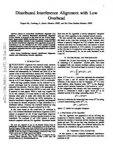
which, again not surprisingly, coincides with the advocated LD approach when x2 + x3 is a lattice point. We conclude that the LZF and the LD approaches correspond to ML decoding under arbitrary interference constrained into some linear subspace, and approximated MAP decoding taking into account the true discrete nature of the interference. IV. P ERFORMANCE It is true that the full rank criteria is almost-surely satisfied for channel coefficients drawn randomly from a continuous distribution. However, in addition to rank criterion, the overall performance of IA with LZF highly depends on the orthogonality of the channel coefficient matrices G1 , G2 , G3 . Notice that the channel matrices are ill-conditioned if two elements of the diagonal matrix T are close in value (and the rank criteria breaks if two elements of T are exactly the same). Further, the channel matrices are also ill-conditioned if the absolute value of any of the channel coefficients deviates from one, especially for larger n. The reason becomes clear by inspecting the exponential structure of the precoding matrices in (2) and the diagonal channel ratio matrix T in (3); if any of the diagonal elements of T have an absolute value lower (or higher) than 1, the corresponding row in V1 exponentially tends to zero (or infinity) for large n. Thus, we expect a poor performance from linear alignment with LZF for dynamic channel amplitudes. Consider first a random channel where channel coefficients t all have magnitude 1 with a random uniform phase, i.e., H √kl = t t exp{jφkl } for i.i.d. φkl ∼ U(0, 2π), k, l = 1, 2, 3, j = −1. For this setup, Fig. 1 shows a simulation comparison between filtering out the interference subspace (LZF), and a nonlinear strategy using Schnorr-Euchner sphere decoding strategy (LD) of [5]. In this figure, the vertical access represents symbol error rate, and the horizontal axis represents average SNR. Here, SNR is defined as the ratio of average transmit power to noise, and is computed by averaging the realized transmit power (including the channel inversion) over a set of consecutive blocks for fixed constellation energy and received noise variance. We compare the linear alignment strategy with LZF, and the discrete alignment scheme with LD, for blocklengths N = 2n + 1 = 21 and N = 2n + 1 = 11. In all simulations, the source symbols are drawn from a 4-QAM (QPSK) constellation. Fig. 1 shows that LD obtains a significant improvement over LZF. As shown in this figure, even with fixed channel

LD, n=5 LZF, n=5 LD, n=10 LZF, n=10 −4

10 −10

0

10

20

30 40 SNR(dB)

50

60

70

80

Fig. 1. Comparison between LZF and sphere lattice decoding (LD) for fixed channel amplitudes. The source constellation is 4-QAM. Dynamic Channel Amplitudes

0

10

−1

10

Symbol Error Rate

x1 ∈C

−2

10

−2

10

−3

10

LD, 0.8