Purdue University
Purdue e-Pubs Open Access Dissertations
Theses and Dissertations
Fall 2014
A nonlinear interface formulation for frictional contact Layla K Amaireh Purdue University
Follow this and additional works at: https://docs.lib.purdue.edu/open_access_dissertations Part of the Civil Engineering Commons Recommended Citation Amaireh, Layla K, "A nonlinear interface formulation for frictional contact" (2014). Open Access Dissertations. 221. https://docs.lib.purdue.edu/open_access_dissertations/221
This document has been made available through Purdue e-Pubs, a service of the Purdue University Libraries. Please contact
[email protected] for additional information.
PURDUE UNIVERSITY GRADUATE SCHOOL Thesis/Dissertation Acceptance Layla Amaireh
A NONLINEAR INTERFACE FORMULATION FOR FRICTIONAL CONTACT
Doctor of Philosophy
Dr. Ghadir Haikal Dr. Ayhan Irfanoglu
Dr. Antonio Bobet
Dr. Eric Nauman
To the best of my knowledge and as understood by the student in the Thesis/Dissertation Agreement, Publication Delay, and Certification/Disclaimer (Graduate School Form 32), this thesis/dissertation adheres to the provisions of Purdue University’s “Policy on Integrity in Research” and the use of copyrighted material. Dr. Ghadir Haikal
Dr. Rao S. Govindaraju
08/14/2014
i
A NONLINEAR INTERFACE FORMULATION FOR FRICTIONAL CONTACT
A Dissertation Submitted to the Faculty of Purdue University by Layla K Amaireh
In Partial Fulfillment of the Requirements for the Degree of Doctor of Philosophy
December 2014 Purdue University West Lafayette, Indiana
ii
To the spirit of my dad, who is the strongest motivation in my life and the foundation of my success. To my husband Mohammad who is the rock and friend of my life, To my joy; my children Leen, Ayah, Abdullah and Ahmad who have been always patient through this journey and handled all my absence from many family occasions with a smile.
iii
ACKNOWLEDGEMENTS
I would like to acknowledge, thank, and express my gratitude to my advisor, Professor Ghadir Haikal, who provided me with the utmost personal support, guidance, encouragement, and intellectual advice through the period of my study. Deep appreciation and thanks are due to Professor Antonio Bobet, Professor Ayhan Irfanoglu, and Professor Eric Nauman, for serving on my dissertation committee and providing me with valuable comments.
Special thanks are due to Dr. Mohammad Alhassan, Dr. Suleiman Ashur, Yazan Khasawneh, Xiaowo Wang, and Hui Liu for their valuable discussions.
I would like to express my eternal gratitude and thanks to my mother and father, my husband and children, my sisters and brothers, my mother and father in law, and my sincere relatives and friends. Their endless supports are indispensable for me to finish this work and in making all this possible. Special thanks are due to my lovely sister Lubna Amaireh for being with me in every step through this tough journey.
iv
TABLE OF CONTENTS
Page LIST OF TABLES ............................................................................................................ vii LIST OF FIGURES ......................................................................................................... viii ABSTRACT
.................................................................................................................. xi
CHAPTER 1. INTRODUCTION......................................................................................1 1.1
Problem Statement .............................................................................................. 1
1.2
Scope of the Research ......................................................................................... 4
1.3
Contents .............................................................................................................. 5
CHAPTER 2. LITERATURE REVIEW ...........................................................................7 2.1
Overview of Available Contact Formulations .................................................... 7
2.2
Algorithmic Treatment of Frictional Contact ................................................... 15
CHAPTER 3. FINITE ELEMENT FORMULATION OF CONTACT ............................ PROBLEMS .............................................................................................18 3.1
Preface............................................................................................................... 18
3.2
Formulation of the Boundary Value Problem ................................................... 18
3.2.1 Equilibrium and Virtual Work .......................................................................19 3.2.2 Large-Deformation Kinematics .....................................................................21 3.2.3 Linearization of the Weak Form ....................................................................23 3.2.4 Discretization .................................................................................................24 3.2.5 Material Laws ................................................................................................26 3.2.5.1 Hyperelasticity ....................................................................................... 26 3.2.5.2 Large-Deformation Plasticity................................................................. 30 3.3
Frictionless Contact .......................................................................................... 38
3.3.1 Definition of the Contact Constraints ............................................................38
v Page 3.3.2 Energy Approach ...........................................................................................40 3.3.3 Enforcing the Contact Constraints .................................................................41 3.3.4 Contact Patch Test Using the Node to Surface Approach .............................42 3.3.5 Interface Model: EDGA ................................................................................45 3.3.5.1 EDGA: The Fully Coupled Case ........................................................... 46 3.3.5.2 EDGA: Contact with Sliding ................................................................. 49 CHAPTER 4. EXTENSION OF THE EDGA FOR PLASTICITY ................................52 CHAPTER 5. FRICTIONAL CONTACT ......................................................................57 5.1
Frictional Contact Formulation ......................................................................... 57
5.2
Enforcing Frictional Contact Constraints ......................................................... 59
5.3
Plasticity-Inspired Approach ............................................................................ 61
5.3.1 Small Deformation Frictional Contact ..........................................................62 5.3.2 Large-Deformation Frictional Contact ..........................................................65 CHAPTER 6. NUMERICAL RESULTS ........................................................................68 6.1
Verification of the Gauss-Kronrod Integration Scheme ................................... 69
6.2
Contact Patch Test ............................................................................................ 71
6.2.1 Small Deformation Linear Elastic Case ........................................................71 6.2.2 Material and Geometric Nonlinearity ............................................................73 6.2.2.1 Large-Deformations, Linear Elastic Material ........................................ 73 6.2.2.2 Large Deformations with Hyperelasticity .............................................. 75 6.2.2.3 Large-Deformation with Von Mises Plasticity ...................................... 76 6.2.2.4 Large-Deformation with Drucker-Prager Plasticity............................... 80 6.3
Sliding Patch Test ............................................................................................. 81
6.3.1 Sliding Patch Test for Hyperelasticity ...........................................................82 6.3.2 Sliding Patch Test for Von Mises Plasticity ..................................................83 6.4
Numerical Examples for Friction...................................................................... 85
CHAPTER 7. CONCLUSIONS AND FUTURE WORK ..............................................93 7.1
Conclusions ....................................................................................................... 93
7.2
Future Work ...................................................................................................... 95
vi Page REFERENCES ..................................................................................................................96 VITA
................................................................................................................102
vii
LIST OF TABLES
Table ..............................................................................................................................Page Table 4.1 Gauss-Kronrod Quadrature Locations and Weights for N=2 ........................... 55
viii
LIST OF FIGURES
Figure .............................................................................................................................Page 3.1 Two Solid Domains in No Contact (Left) and Contact (Right) Configurations ......... 19 3.2 Kinematics of a Continuum Body (Bonet and Woods, 2008) .................................... 22 3.3 Multiplicative Decomposition (Bonet and Woods, 2008) .......................................... 30 3.4 Radial Return Mapping (Bonet and Wood, 2008) ...................................................... 33 3.5 FEM Interface Discretization. ..................................................................................... 38 3.6 Gap Function............................................................................................................... 39 3.7 Kuhn-Tucker Conditions (Left) and Contact Forces vs. Normal Gap (Right) ........... 40 3.8 Contact Patch Test ...................................................................................................... 42 3.9 Complete Transfer of Stresses Through the Interface in Conforming Meshes (Left) Versus Incomplete Transfer of Stresses in Non-Conforming Meshes (Right) ............................................................................................................ 44 3.10 Local Enrichment of the Interface Element for the Following Cases: (a) Single Node, (b) Multiple Nodes, and (c) Added Node Reference in the Parent Domain (Haikal, 2009)......................................................................... 46 3.11 Contact Patch Test with EDGA ................................................................................ 49 3.12 Enrichment Updating Procedure for Sliding (Haikal, 2009) .................................... 50 4.1 Q4 Element with Gauss Quadrature Integration Points Inside(Left) and the Enriched Element with Gauss-Kronrod Integration Points (Right) .................... 54 4.2 Q4 Element with Gauss Quadrature Integration Points at the Interface (Left) and the Enriched Element with Gauss-Kronrod Integration Points (Right) .............. 54 6.1 Patch Test for Q4 Element with Enrichment (Left) and the Gauss-Kronrod Quadrature Integration Points in the Parent Element (Right) ..................................... 69 6.2 Stress Distributions for Q4 Element with Gauss-Kronrod Integration Points ............ 70
ix Figure .............................................................................................................................Page 6.3 Deformed Shape for Q4 Element with Gauss-Kronrod Integration Points ................ 70 6.4 Contact Patch Test for the Small Deformation Linear Elastic Case: Deformed Shape without EDGA(Left) and with EDGA(Right) ................................ 72 6.5 Contact Patch Test for the Small Deformation Linear Elastic Case: Stress Field without EDGA (Left) and with EDGA(Right)........................................ 72 6.6 Contact Patch Test for the Linear Elastic Case: Deformed Shape without EDGA (Left) and with EDGA (Right)........................................................................ 74 6.7 Contact Patch Test for the Linear Elastic Case: Stress Field without EDGA (Left) and with EDGA(Right) ................................................................................... 74 6.8 Contact Patch Test for the Nonlinear Elastic Case: Deformed Shape without EDGA(Left) and with EDGA(Right) ........................................................................ 75 6.9 Contact Patch Test for the Nonlinear Elastic Case: Stress Field without EDGA (Left) and with EDGA (Right) ...................................................................... 76 6.10 Contact Patch Test for the Elasto-Plastic Case (Von Mises): Deformed Shape without EDGA(Left) and with EDGA the Extension for Plasticity (Right) ............. 77 6.11 Contact Patch Test for the Elasto-Plastic Case (Von Mises): Stress Field without EDGA (Left) and with EDGA and the Extension for Plasticity (Right)...... 77 6.12 Contact Patch Test for the Elasto-Plastic Case (Von Mises) .................................... 79 6.13 Contact Patch Test for the Elasto-Plastic Case (Von Mises): Stress Field (Left) and with EDGA and the Extension for Plasticity (Right) ............................... 80 6.14 Contact Patch Test for Elasto-Plastic Case (Drucker-Prager): Deformed Shape without EDGA (Left) and with EDGA and the Extension for Plasticity (Right)...... 80 6.15 Contact Patch Test for Elasto-Plastic Case (Drucker-Prager): Stress Field without EDGA (Left) and with EDGA and the Extension for Plasticity(Right)....... 81 6.16 Sliding Patch Test ..................................................................................................... 81 6.17 Sliding Patch Test for the Nonlinear Elastic Case: Deformed Shape without EDGA (Left) and with EDGA (Right) ...................................................................... 82 6.18 Sliding Patch Test for the Nonlinear Elastic Case: Stress Field without EDGA (Left) and with EDGA (Right) ...................................................................... 83
x Figure .............................................................................................................................Page 6.19 Sliding Patch Test for Von Mises Plasticity Case: Deformed Shape without EDGA (Left) and with the Extension of the EDGA (Right) ........................ 84 6.20 Sliding Patch Test for Von Mises Plasticity Case: Stress Field without EDGA (Left) and with the Extension of the EDGA (Right) ..................................... 84 6.21 Incremental Deformation for Numerical Example 1 ................................................ 86 6.22 Geometry and Loading Conditions for Numerical Example 2 ................................. 87 6.23 Deformed Shape for Numerical Example 2 .............................................................. 88 6.24 Horizontal Stress Distribution for Numerical Example 2 ......................................... 88 6.25 Normal Stress Distribution for Numerical Example 2 .............................................. 89 6.26 Tangential and Normal Stresses along the Interface for Numerical Example 2 ....... 89 6.27 Geometry and Loading Conditions for Numerical Example 3 ................................. 91 6.28 Deformed Shape for Numerical Example 3 .............................................................. 91 6.29 Horizontal Stress Distribution for Numerical Example 3: Our Approach (left) versus ABAQUS (right) .................................................................................. 92 6.30 Normal Stress Distribution for Numerical Example 3: Our Approach (left) versus ABAQUS (right) .................................................................................. 92 6.31 Tangential and Normaal Interface Stresses Along the Interface for Numerical Example 3 ................................................................................................ 92
xi
ABSTRACT
Amaireh, Layla K. PhD, Purdue University, December 2014, A Nonlinear Interface Formulation for Frictional Contact. Major Professor: Ghadir Haikal. Finite element simulations of contact problems often involve modeling the interaction of multiple bodies across a non-confirming interface. Non-Confirming Meshes (NCM) are typically associated with large sliding or adaptive refinement on one side of the interface to capture localized nonlinear behavior due to large deformations, damage and inelasticity. The use of NCMs, however, presents a number of numerical issues; the main challenge with such discretizations is to ensure compatibility of the kinematic and traction fields along the non-conforming interface. The Enriched Discontinuous Galerkin Approach (EDGA) (Haikal and Hjelmstad,2010)addresses this challenge by implementing a local enrichment along with an interface stabilization procedure, based on the Discontinuous Galerkin formulation, to enable a two-pass approach in enforcing contact conditions that preserves the weak continuity of surface tractions without introducing dual interface fields. In this study, the Enriched Discontinuous Galerkin Approach (EDGA) is extended to model contact in the presence of material and geometrical nonlinearities, as well as friction. The enrichment used in the EDGA introduces a higher-order interpolation on the contact interface, which requires an increase in the integration rule. To avoid changing
xii the integration point locations to accommodate the higher-order interpolation we employ a progressive integration rule (Gauss-Kronrod quadrature) that preserves material history at existing integration points. A new approach for handling frictional conditions under large deformations is introduced. The proposed approach is designed to increase algorithmic efficiency and circumvent numerical issues encountered when modeling stick/slip conditions in Coulomb frictional contact models.
1
CHAPTER 1. INTRODUCTION
1.1
Problem Statement
With the advent of powerful computing, the Finite Element Method (FEM) has become a popular tool for simulating the behavior of many complex engineering systems with a high level of detail. Computational models for contact problems, in general, and frictional contact problems, in particular, are in high demand in structural engineering and many other fields, where the accurate modeling of the interaction between different components across interfaces is required to simulate the behavior of systems such as steel connections, bridge bearings, soil-structure interaction in piles or other foundations, among others. In modeling contact problems, if the bodies coming into contact are discretized using different finite element meshes, or in the presence of large sliding, the nodes from the first body will no longer coincide with those of the second body across the interface, therefore resulting in anon-conforming mesh (NCM). A NCM mesh, by definition, is a finite element discretization of a given domain where point-wise displacement continuity does not hold along a given interface separating two domains discretized with conforming meshes. NCM are created by large sliding or when different finite element mesh sizes are used to increase accuracy in capturing the behavior in each component and/or along the interface. Interface behavior can be unilateral, as is typical in contact
2 problems where the two bodies are allowed to separate from each other, or bilateral ensuring full coupling regardless of loading/deformation conditions. The main challenge in both cases, however, is to ensure deformation compatibility and continuity of interface tractions in the absence of full displacement conformity along the interface. The difference between unilateral contact and bilateral coupling is that these conditions apply to the normal components of the kinematic and traction fields, only, in unilateral contact. As such, methods for unilateral contact and bilateral coupling have traditionally been used interchangeably. Previous studies used different techniques to resolve the challenge of enforcing interface conditions in NCMs, with varying levels of success, as will be discussed below. Additional complications arise in the presence of friction, as well as geometric and material nonlinearities. These complications have led to a number of numerical issues in the resolution of contact problems, including interface locking, loss of stability, incomplete interface pressure fields, among others (Sheng et al., 2006). Contact formulations are generally classified into primal and dual methods, based on the nature of the interface variables. Dual methods, including the popular mortar method (Puso and Laursen, 2004), use the tractions as an interface variable and employ a dual field of Lagrange multipliers to enforce weak geometric compatibility at the interface. The Lagrange multipliers at the nodes along one side of the interface, called “slave” are computed in terms of the interpolated field based on the other side of the interface, called “master.” Dual methods satisfy the continuity of interface tractions, typically reflected in the contact patch test, by design. The master/slave designation, however, is not always trivial and has a direct impact on the result. Furthermore, the
3 choice of the Lagrange multiplier interpolation field is restricted by the LadyzhenskayaBabuška-Brezzi (LBB) condition that governs the stability of dual finite element discretizations. In primal methods, the interface is represented by its displacement fields; therefore, these approaches are not subject to the LBB restrictions. Primal methods, however, are challenged by the task of enforcing both geometric compatibility and continuity of the tractions using a primal variable field. The fact that the discretization is pre-determined by NCM adds to this challenge. As a result, primal methods, including the popular Discontinuous Galerkin (DG) and Nitsche (Nitsche, 1971) approaches, often require a mesh-dependent stabilization parameter to ensure the convergence of the solution in the limit of mesh refinement. The properties of stability and convergence, however, can only be guaranteed for linear problems. An exception to this observation is the Enriched Discontinued Galerkin Approach (EDGA) formulation proposed by (Haikal and Hjelmstad, 2010) for linear elasticity. The EDGA employs a local enrichment to transform the node-to-surface contact constraints to node-to-node, thereby enabling a two-pass approach in the treatment of contact conditions. Another key feature of the formulation is its ability to enforce traction continuity across the interface. The objective of this thesis is to propose a novel contact formulation for solving general contact problems with NCMs in the presence of material nonlinearity, including plasticity, in a large deformations setting, by developing an interface finite element model that ensures geometric compatibility and complete transfer of surface tractions between the domains of the contact problem. The proposed method is based on the Enriched Discontinued Galerkin Approach(EDGA) formulation proposed by Haikal and Hjelmstad
4 (2010) for the case of linear elasticity. We extend the EDGA to the case of plasticity using the Von Mises and Drucker-Prager yield criteria and address some of the issues pertaining to the integration of plastic internal variables. We also propose a new plasticity-inspired formulation for large-deformation frictional contact of hyperelastic bodies. This research has many critical applications in structural, mechanical, and biomedical engineering, such as soil-structure interaction, composite materials, tire-road interaction, and biomechanical systems such as joint replacements. The use of conventional finite element techniques without accurate consideration of the involved contact interactions may result in erroneous results leading to costly and immature failure in these systems.
1.2
Scope of the Research
The scope of this research includes the following main tasks: (a) Formulation of the coupled problem: this includes the formulation of the boundary value problem (equation of motion, large-deformation formulation, and constitutive models) and the contact treatment with and without friction. The Newton method is used to solve the nonlinear system of equations. (b) Application of the EDGA with and without sliding: the EDGA is a primal interface formulation based on two key procedures: a local enrichment of interface primal variables and stabilization of tractions along the interface. The enrichment is used to enforce geometric compatibility in an unbiased manner by transferring the continuity constraint from node-to-surface to node-to-node. The
5 stabilization procedure is based on the Discontinuous Galerkin (DG) method and is used to ensure a complete transfer of the tractions field across the interface. (c) Extension of the EDGA to the case of plasticity, using the Von Mises and Drucker-Prager material models. (d) Frictional contact: A new plasticity-inspired formulation for large-deformation frictional contact under hyperelasticity conditions is proposed. (e) Verification and numerical studies: the patch test is used to verify that the proposed formulation reflects a complete transfer of tractions and geometric compatibility at the interface, for frictional and frictionless contact cases. Additional numerical examples are used to demonstrate the effectiveness of the proposed formulation and compare the results with the literature.
1.3
Contents
This thesis consists of five chapters. Chapter 1 (Introduction) presents the problem statement and motivation behind the investigation and development of the proposed formulation. Chapter 2 (Literature Review) includes an extensive critical review of available modeling approaches for simulation of contact problems. The advantages and disadvantages of different methods are discussed. Chapter 3 (Finite Element Formulation) includes: (1) the formulation and implementation of the boundary value problem for both frictionless and frictional contact in the presence of large deformations and material nonlinearity, and (2) the formulation and implementation of the EDGA for bilateral and unilateral coupling (with and without sliding). Chapter 4 (Extension of the EDGA for Plasticity) presents an extension of the EDGA for large-
6 deformation plasticity. Chapter 5 (Frictional Contact) discusses the implementation of frictional contact conditions and presents a new plasticity-inspired formulation for largedeformation frictional contact of hyperelastic bodies. Chapter 6 (Numerical Results) presents numerical results that illustrate the effectiveness of the developed approach for both frictionless and frictional contact cases. Chapter 7 (Conclusions and Future Work) includes conclusions drawn based on the findings of this work and recommendations for future work.
7
CHAPTER 2. LITERATURE REVIEW
In this chapter, we conduct a thorough literature review to document and discuss previous research in the area of contact problems in general, and frictional contact problems in particular. We focus on relevant studies that discussed or utilized systematic techniques for modeling unilateral contact as well as bilateral coupling in nonconforming meshes (NCM) problems, including those developed for particular applications, such as soil-structure interaction. The methodologies, conclusions, and recommendations of the previous works were considered in formulating the objectives, scope, and methodology of this thesis.
2.1
Overview of Available Contact Formulations
As mentioned in section 1.1, contact formulations can generally be grouped into two main categories: primal and dual methods. Dual methods use the traction field as an interface variable and they employ a field of Lagrange multipliers, based on the master side of the surface, to enforce geometric compatibility at the interface. These methods are therefore inherently biased and the choice of the Lagrange multiplier field and are subject to the LBB conditions. In primal methods, the interface is represented by its displacement fields. Therefore, primal methods are not subject to the LBB restrictions. These methods, however, are challenged by the task of enforcing both geometric compatibility and
8 continuity of the tractions using a primal variable field. The fact that the discretization is pre-determined by the NCM adds to the complexity of this challenge. The earliest and simplest contact formulation is the node-to-surface method that enforces the displacement continuity between a set of slave nodes at one side of the interface and their projections along the opposing master surface using a set of discrete Lagrange multipliers. This method is generally not capable of representing a state of constant pressure and therefore fails the well-known patch test (Papadopoulos and Taylor, 1992). The primal interface element method was widely used in the literature. Zaman et al. (1984) developed a simple thin-layer element and used it in a finite element procedure for simulation of various modes of deformation in dynamic response. The isoparametric interface element is compatible with both domains, and has a simple constitutive law with constant values for both shear and normal stiffness. The authors believed that the proposed element could provide satisfactory and consistent formulation of interface behavior under dynamic loading. However, they stated that in view of the complexity of the problem and influence of a number of factors, such as geometry, type of loading, material properties, time integration, and mesh layouts, further investigations will be needed in order to delineate their effects on the dynamic response. Hird and Russell (1990) presented an analytical solution for the compression of a long elastic block, bonded along one side to a rigid material. Numerical results showed a good agreement with the analytical solution. Karadeniz (1999) introduced an interface 3-D beam element for the analysis of framed structures, which interact with an elastic medium. The formulations of the element were based on the assumption that the elastic medium can be
9 represented by a two-parameter model of the Winkler model and Pasternak model (Pasternak, 1954). Luan and Wu (2004) proposed a nonlinear elasto-perfect plastic model for the interface element to simulate the behavior of Soil-Structure-Interaction (SSI) contact problems. The stress-strain relationship and nonlinear elasto-perfect plastic matrix of interface element were established based on elasto-plasticity theory. It was indicated that the proposed model can rationally simulate the stress-strain relationship of the interface element and will be practically applicable. Swamy et al. (2011) analyzed SSI problems adopting the finite element method, and the usage of link/interface elements between two elements of different materials. The study concluded that the presence or absence of interface elements affects the settlement, differential settlements and stresses in soil. Also, the interface element plays a crucial role in nonlinear analysis when constitutive relations of soil depend on the state and increment of stress and strain. Mahmood et al. (2008) adopted a finite element approach to model a SSI system that consists of reinforced concrete plane frame, soil deposit, and interface, which represents the frictional surface between foundation of the structure and subsoil. The authors concluded that the thin-layer interface element method could successfully simulate the effect of slip and separation in the dynamic analysis of soil-reinforced concrete frame interaction problems. This technique is able to take into account the nonlinearity of the material, but it is not applicable in case of large-deformation problems. The domain decomposition method for modeling coupled nonlinear problems is based on the solution of a boundary value problem consisting of two domains, a finite domain representing the structure and a semi-infinite domain representing the soil into which the structure is embedded. These two domains are separated by a boundary called
10 the interface. The aim of solving the boundary value problem is to determine the displacements and stresses in both domains numerically or using the finite element method. The main advantage of this method is its capability to solve nonlinear boundary value problems with arbitrary geometry, boundary conditions and constitutive properties. Lai et al. (1991) presented an iterative process based upon a hybrid residual force method for solving elasto-plastic contact problems. In this approach the domains are treated as separate bodies and related only by compatibility of displacements and equilibrium of forces at the interface. This scheme leads to a significant improvement in numerical stability and rate of convergence over the conventional initial stress method. Yazdchi et al. (1999) presented a study on the transient response of an elastic structure embedded in a homogeneous, isotropic and linearly elastic half-plane. Transient dynamic and seismic forces were considered in the analysis. The numerical method employed was the coupled Finite-Element–Boundary-Element technique (FE–BE). Finite element method (FEM) was used for discretization of the near field and the boundary element method (BEM) was employed to model the semi-infinite far field. These two methods were coupled through equilibrium and compatibility conditions at the interface. The results of the analysis showed the importance of including the foundation stiffness and thus the dam– foundation interaction. It was shown that the coupled FE–BE method is efficient, accurate and versatile. Rizos and Wang (2002) presented a coupled BEM-FEM methodology for 3D wave propagation and contact analysis in the direct time domain. The employed BEM uses a new generation of the Stokes fundamental solutions that utilize the B-Spline family of polynomials. A standard finite element methodology for dynamic analysis along with direct integration in time was coupled to the BEM through a
11 staggered solution approach. Jahromi et al. (2009) proposed the domain decomposition method for modeling coupled nonlinear contact problems. The method assumes that the coupled system is physically partitioned into independently modeled sub-domains. A coupling procedure based on the sequential iterative Dirichlet-Neumann coupling algorithm was used, which utilizes the condensed tangent stiffness matrices at the interface to ensure and accelerate convergence to compatibility in successive update of the boundary conditions. A limitation of this method is that problems involving nonhomogeneous and nonlinear domains result in a more complicated solution procedure. The mortar method (otherwise known as the segment-to-segment formulation) is a widely used dual approach, where the gap function is averaged along the contacting segments and the pressure at the slave contact points is interpolated in terms of the nodal pressures on the master surface (Puso and Laursen, 2004). The drawback in this method is the LBB limitation as well as the bias of choosing the master and slave surfaces. The finite elements method and direct finite elements method can used to analyze and solve contact problems. Erxiang et al. (1998) analyzed a nonlinear dynamic interaction problem of saturated soil and structure by using the direct finite element method. The study proposed a model that combines the well-established Mohr-Coulomb model for the soil plasticity and a densification model for the pore pressure build up. Performed calculations showed the efficiency of this approach. The authors stated that the accuracy seems acceptable; however, it still requires some research into its application when nonlinearity exists close to the artificial boundary. Wang et al. (2004) developed a finite element model to simulate nonlinear response of piles/drilled piers under axial loading. It was found that an accurate undrained shear strength profile is of
12 the highest importance for the capacity analysis. Proper account of over consolidated crust is important especially for short pier capacity simulation, while nonhomogeneity of undrained shear strength distribution is not critical for the stiff clay site. Park et al. (2007) introduced a method for contact analysis by adopting an unaligned mesh generation approach and using a direct method with modified Lysmer transmitting/absorbing boundary (Lysmer, 1969) where soil media is modeled to uniform structured finite elements with discontinuity. They found that the variation of the peak value changes largely due to the soil profile and properties. Lu et al. (2004) employed a new parallel nonlinear finite element program (ParCYCLIC) in order to satisfactorily reproduce the SSI effects under earthquake loading. A single pile embedded in mildly inclined, liquefiable soil deposit was analyzed under dynamic base shaking conditions. Huo et al. (2005) investigated the earthquake related failures of the Daikai Station. A numerical dynamic analysis using ABAQUS of the structure and the surrounding soil was conducted using motions accelerations recorded near the site as input. They concluded that the use of seismically induced free-field deformations for structural design is only a first approximation, which requires further evaluation for sensitive structural members in underground structures. A stronger interface will be able to transmit larger shear to the structure but will induce more confinement to the surrounding soil thus limiting its shear modulus degradation. Sheng et al. (2007) demonstrated the application of computational contact mechanics in strip footing under eccentric and inclined loads and a cone penetration test. They presented a general formulation for problems involving frictional contact and a general description of the associated numerical algorithms. It was recommended that Soil-Structure-Interaction (SSI) contact systems that involve large
13 deformations and surface separation and re-closure, are in general better represented by frictional contact than prescribed boundary conditions or joint elements. Liao et al. (2007) studied the SSI contact problem on loose ground using the advanced nonlinear finite element analysis software MSC. Marc. The study concluded that peak accelerations of ground surface decrease because of the effects of SSI; the thicker the soil is, the smaller the decrease scale is. Sheng et al. (2008) introduced a modified finite element formulation of frictional contact for soil-pile interaction. The formulation was based on smoothed discretization of the pile surface using BEZIER polynomials. The results showed that the new finite element formulation can produce reasonable results for the pile loading problem that involves large interfacial sliding and surface separation. The drawback in this method is the bias of choosing the master and slave surfaces. Paknahad et al. (2008) investigated modeling of a shear wall structure-foundation and soil system using the super element, finite and infinite elements while considering soil nonlinearity. The applicability of the proposed idealization was shown through analyzing a shear wall structure under static loadings. Gul et al. (2009) presented the extension of the Direct Differentiation Method (DDM) to finite element models with node-to-surface contact. The DDM is an accurate and efficient method for computing finite element response sensitivities to material, geometric and loading parameters. The developments presented in this study close an important gap between finite element response-only analysis and finite element response sensitivity analysis through the DDM, extending the latter to applications requiring response sensitivities using finite element models with node-tosurface constraints Such applications include structural optimization, structural reliability analysis, and finite-element model updating.
14 One of the most widely primal coupling approaches is the Discontinuous Galerkin (DG). This approach is used for the coupling problem since it readily assumes discontinuous discretization on all inter-element interfaces. The DG formulation (Brezzi et al., 1999) is based on identifying a set of target continuous fields for the displacement and traction fields on each interface, and mapping the discretized displacement and traction fields on each surface to these target fields in a weak weighted residual form. Another primal method is the Nitsche method (Nitsche, 1971) that is a consistent primal formulation that employs a penalty approach to enforcing kinematic conditions. Originally introduced for the treatment of rough Dirichlet boundaries, the Nitsche method has been used as a basis for developing primal stabilized interface formulations for embedded interfaces. The clear advantages of the primal DG and Nitsche methods over dual ones are the unbiased treatment of the interface and the absence of the LBB restrictions. These methods, however, require a mesh-dependent stabilization parameter. The Enriched Discontinuous Galerkin Approach (EDGA) developed by Haikal and Hjelmstad (2010) for the coupling of NCM is a primal interface formulation that ensures geometric compatibility and a complete transfer of surface tractions between the connecting elements at the non-conforming interfaces. The approach is based on a local enrichment of the non-conforming interface that enables a simple enforcement of the continuity of the displacement field using a set of discrete node-to-node constraints, thereby eliminating the need for master/slave designations. The authors treated the interface using a form of the Discontinuous Galerkin (DG) method that guarantees the complete transfer of forces along non-conforming inter-element boundaries. The proposed interface formulation was shown to be consistent, stable and includes the
15 continuous Galerkin as a subset. The key advantages of this method are that it uses finite element estimates of the stress fields on the interface, and it is able to accommodate sliding and nonlinearity (material and geometric). As can be noticed from the literature review, previous studies used different techniques to resolve the interface problem in systems in contact. The used techniques have shown major drawbacks such as: the inability of combining the material nonlinearity and the geometric nonlinearity, or have complicated procedures when the problem involves nonlinearity. The importance of this work stems from the lack of a finite element model that is capable of addressing with enhanced accuracy, the nonlinearity in the material, large deformations and friction on the interface with NCM. The emphasis in this research is on the interface model such that it is capable of capturing accurate behavior of each component of systems in contact without any bias. The EDGA was developed for the case of hyperelasticity, and in this study we extend the EDGA to model contact problems with plasticity. We assume large deformations and nonlinear constitutive models for both domains. The presence of friction and sliding will also be taken into account.
2.2
Algorithmic Treatment of Frictional Contact
Enforcing the contact constraints in the presence of friction requires distinguishing between stick and the slip states within each load step, which requires enforcing or releasing the tangential constraints. Stick conditions can be enforced with the same approaches used for normal contact constraints, namely the Penalty, Lagrange multiplier, or Augmented Lagrangian methods.
16 The Lagrange multiplier method is used to enforce exact stick conditions. However it introduces an extra unknown, therefore increasing the size of the problem, and may also lead to scaling-related convergence difficulties (Vulovic et al., 2007). The penalty method is widely used due to its simplicity and since it does not introduce an extra unknown. This method introduces a force at the contact locations, controlled by a penalty parameter, to eliminate the penetration at the interface. The challenge in using the penalty method, however, is in identifying the magnitude of the penalty parameter: A large parameter is needed to preclude penetration. Arbitrarily large values, however, could potentially lead to ill-conditioning and instability (Vulovic et al. 2007 and Ştefancu et al. 2011). The Augmented Lagrangian method combines the benefits of the penalty and Lagrangian multiplier approaches. The contact force is computed through an iterative process starting with a penalty-based estimate. This method has the advantage of obtaining the exact Lagrange multiplier values and avoiding the numerical problems associated with the penalty approach (Simo and Laursen, 1992, Laursen and Simo, 1993a, Wriggers and Zavarise, 1993, and Pietrzak and Curnier, 1999). It remains, however, an iterative process, much like the Lagrange multiplier approach, that requires an initial assumption of stick/slip at each contact point. When the above methods are used to enforce Coulomb frictional conditions, an assumption has to be made at the onset of the simulation, whether contact at a given point is in stick or slip. If a stick condition is assumed, the lateral force is computed that is required to enforce zero tangential displacement. This assumption has to be revisited at the end of the analysis, and if the force is found to be in excess of the Coulomb frictional limit, set to be equal to the normal force multiplied by the surface friction coefficient, the
17 stick condition has to be revised to allow tangential slip, and the solution has to be repeated under the revised assumption. For large meshes, and under material and/or geometric nonlinearity, this process requires multiple repetitions of the solution of the nonlinear equilibrium equations of the coupled system. The change in stick/slip conditions at multiple contact nodes could also be the source of lack of convergence or instability (Sheng et al., 2006). Another method used to enforce frictional contact conditions uses the elastoplasticity analogy in formulating the nonlinear constitutive equations of friction. The tangential displacement is decomposed into elastic or reversible (stick) and plastic or irreversible (slip) parts. The tangential traction forces are computed as the forces required to enforce the stick condition. If these forces exceed the maximum value allowed by the Coulomb model, lateral displacement occurs through “plastic” slip and the tangential traction is computed through a return mapping algorithm with an associative flow rule for the tangential displacement. This approach has a tangible physical interpretation; the stick condition represents the elastic part of the tangential displacement at the contact location that vanishes when the loading is removed, while the slip condition represents the irrecoverable part of the displacement. The method eliminates the convergence problem and the need for repeated nonlinear solutions caused by enforcing and releasing the contact constraints. This method showed effectiveness in linear elastic problems, however applying it in the context of large deformations has proven to be a challenge (Laursen and Simo, 1993b, Sheng et al., 2006, and Masud et al., 2012).
18
CHAPTER 3. FINITE ELEMENT FORMULATION OF CONTACT PROBLEMS
3.1
Preface
The formulation of interface problems involves ensuring geometric compatibility and a complete transfer of forces along the interface. In unilateral frictionless contact problems, the bodies are allowed to separate and slide tangentially with respect to each other. Therefore, the continuity condition applies to the normal component of the displacement and traction fields only. In the frictional case, the tangential relative motion between two points in contact is governed by the frictional law, which will be assumed to follow the Coulomb model. For the sake of simplicity, we will begin our presentation of the mathematical formulation of the contact problem assuming that the two contacting domains are fully coupled and remain such throughout deformation. We will then modify the formulation to account for frictionless sliding and frictional conditions on the interface.
3.2
Formulation of the Boundary Value Problem
This section includes the mathematical formulation of the equations of motion, large-deformation kinematics, and material laws. In large-deformation contact problems, the nonlinear relationship between the displacements and strains as well as between the stresses and strains cannot be ignored.
19 Equilibrium between the internal and external forces should also be enforced in the deformed configuration. The formulation of large-deformation problems can be carried out using the total or updated Lagrangian frameworks, with the governing equations written with respect to the initial configuration in the total Lagrangian formulation and with respect to the current configuration in the updated Lagrangian formulation. In the next section, a brief description of the updated Lagrangian formulation is presented; detailed derivations can be found in Bonet and Woods (2008).
3.2.1
Equilibrium and Virtual Work
Consider the two solid domains in contact Ω1 and Ω2shown in Figure 3.1. The boundary Γ of each domain can be divided into three parts Γ =Γt ∪ Γu ∪ Γ, where Γt and Γu denote the Neumann and Dirichlet parts of that boundary, respectively, and Γc refers to the contact interface. Note that Γt ∩ Γu ∩ Γc = Φ in each body.
Figure 3.1 Two Solid Domains in No Contact (Left) and Contact Configurations (Right)
Given the body force vector field for each solid b1 and b2, a prescribed traction t1 and t2on Γt1 and Γt2, and a prescribed displacement field g1 and g2 on Γu1 and Γu2, the
20 strong form of the governing equations of the continuum contact problems can be written as follows: div σ1+ b1 = 0 in Ω1
σ1n = t1 on Γt1
u1 = g1 on Γu1
div σ2+ b2 = 0 in Ω2
σ2n = t2 on Γt2
u2 = g2 on Γu2
and u1=u2,
t1+ t2=0 on Γc,
where σ is the Cauchy stress tensor, div is the divergence operator and n is the normal to the surface. Defining the space T= {u ∈ H1(Ω) : u = g on Γu} and V = { u ∈ H1(Ω) : u = 0 on Γu}; let 𝐮! and 𝐮! be the virtual displacements for domains Ω1and Ω2, respectively, where: 𝐮! ∈ V1= {u! ∈ H1(Ω1): u! = 0 on Γu1} 𝐮! ∈ V2 = {𝐮! ∈ H1(Ω2) : 𝐮! = 0 on Γu2} 𝐮! ∈ Vc= {u! ∈ H1/2(Γc)} The total virtual work done by the system is the sum of the virtual work done by the two bodies in addition to the work done by the contact forces at the interface. Therefore the weighted residual form of the governing equations is: Ω1
Γ2t
𝑑𝑖𝑣 𝛔1 + 𝐛1 . 𝐮1 dΩ + 𝐭2 − 𝛔2 𝐧2 . 𝐮2 dΓ −
Γ1t
ΓC
𝐭1 − 𝛔1 𝐧1 . 𝐮1 dΓ +
Ω2
𝑑𝑖𝑣 𝛔2 + 𝐛2 . 𝐮2 dΩ +
𝐭1 + 𝐭2 . 𝐮 dΓ = 𝟎 ∀ 𝐮 ∈ 𝑉
(3.1)
Applying the divergence theorem to the terms div σ1 on dΩ1 and div σ2 on dΩ2 in Equation (3.1) and imposing homogeneous boundary conditions yields the following:
G(u, u ) = G(u, u )1 + G(u, u ) 2 + G(u, u ) C
(3.2)
21
G(u, u )1 = − ∫ σ1 : ∇u 1dΩ + ∫ t1 ⋅ u 1dΓ + ∫ b1 ⋅ u 1dΩ
(3.3)
G(u, u ) 2 = − ∫ σ 2 : ∇u 2 dΩ + ∫ t 2 ⋅ u 2 dΓ + ∫ b 2 ⋅ u 2 dΩ
(3.4)
1
1
Ω
Ω
1
Γ
2
Γ
Ω
2
Ω
[
2
]
G(u, u ) C = ∫ t1 ⋅ u1dΓ + ∫ t 2 ⋅ u 2 dΓ − ∫ t1 + t 2 ⋅ u dΓ ΓC1
ΓC2
Ω
2
(3.5)
It is important to note that, when t 1 = t 2 , the interface work term G(u, u ) C disappears leaving the total virtual work G(u, u ) = G(u, u )1 + G(u, u ) 2 , which is the sum of the work done in each domain, as is case for conforming meshes. Therefore, it can be concluded that when the displacement field is conforming, the equilibrium of tractions holds automatically on the interface.
3.2.2 Large-Deformation Kinematics Consider a deformable body moving from an undeformed to a deformed configuration as shown in Figure 3.2. Let X and x denote the material and spatial position vectors of any material point p, respectively. The deformation gradient F can be defined as: F = ∇ X x = ∂x ∂ X . The deformation can be expressed by a measure of change in length, represented by the scalar product of any two spatial vectors at a point within the body as: dx1 ⋅ dx 2 = dX1 ⋅ C dX 2 , or dX1 ⋅ dX 2 = dx1 ⋅ b -1dx 2 where C = F T F and b = FF T are the right and left CauchyGreen deformation tensor, respectively.
22
Figure 3.2 Kinematics of a Continuum Body (Bonet and Woods, 2008)
The change in the spatial scalar product can be found in terms of the material and spatial vectors as follows:
1 1 dx ⋅ dx 2 − dX1 ⋅ dX 2 = dX1 ⋅ E dX 2 ; 2
(
)
1 1 dx ⋅ dx 2 − dX1 ⋅ dX 2 = dx1 ⋅ e dx 2 ; 2
(
)
E= e=
1 (C − I ) 2
1 I − b −1 2
(
)
(3.6)
(3.6)
where E is the Lagrangian or Green strain tensor, and e is the Eulerian or Almansi strain tensor. As the body deforms, its volume and area will change, and the magnitude of the change can be computed as: dv = JdA , da = J F −1dA , with J = det F . In these equations, v and V are the volume in the initial and current configurations, respectively; a and A are the area of the initial and current configuration, respectively.
23 The weak form of Equations (3.2) and (3.3) can be written in the current configuration using the Cauchy stress tensor (σ) and its conjugate (∇ u ) as follows:
G (u, u ) = ∫ σ : ∇ u dΩ − ∫ b : u dv − ∫ t : u dΓ Ω
Ω
(3.8)
Γt
or, equivalently:
G (u, u ) = ∫ σ : ε dΩ − ∫ b : u dv − ∫ t : u dΓ ; Ω
Ω
Γt
1 ε = (∇u + ∇u T ) 2
(3.9)
Note that, unless otherwise noted, the gradient operator is defined with respect to the spatial coordinates x. The first term in Equation (3.9) represents the internal virtual work
(WI = ∫ σ : ε dΩ) , whereas the second and third terms represent the external virtual work Ω
done by the applied forces (WE = ∫ b : u dv + ∫ t : u dΓ) . Ω
3.2.3
Γt
Linearization of the Weak Form
In order to obtain the solution of the nonlinear virtual work equation, we implement the Newton-Raphson method and thus linearize the virtual work form as follows:
Gˆ (u, u ) = G (u, u ) + D G (u, u ) ⋅ Δu
(3.10)
The first term in Equation (3.10) is the sum of internal and external work at a displacement estimate u, while the second term represents the directional derivative of the virtual work functional with respect to an increment Δu , and can be computed as:
D G(u, u ) ⋅ Δu = D WI (u, u ) ⋅ Δu + D WI (u, u ) ⋅ Δu = u ⋅ [K (u)Δu − f ]
(3.11)
24 where K(u) is the tangent stiffness matrix and f is the equivalent load vector. For the updated Lagrangian, the directional derivative of the internal virtual work yields:
⎡ ⎤ D WI (u, u ) ⋅ Δu = D ⎢ ∫ σ : ε dΩ⎥ ⋅ Δu ⎣Ω ⎦ 1 = ∫ ε : [z ⋅ Δε ] dΩ + ∫ σ : ∇Δu T ∇ u + ∇ u T ∇Δu dΩ 2 Ω Ω
[
(3.12)
]
−1 where, Δε = (∇Δu + ∇Δu T ) / 2 and zijkl = J FiI F jJ FkK FlL Z IJKL .
The terms ZIJKL and zijkl are the fourth-order material and spatial elasticity tensor, respectively, and will be discussed in detail in the material laws sections.
3.2.4
Discretization
In the finite element method he domain is discretized into a finite number of subdomains, each of which is referred to as the element. Discretization is established in the undeforrmed configuration using isoparametric mapping to a parent element in the reference coordinates ξ. Defining the total number of nodes in each element as n and the shape functions as N, the material and spatial coordinates in the element can be n
interpolated in terms of the corresponding nodal variables as: X = ∑ N α (ξ )Xα , α =1
n
x = ∑ N α (ξ )xα . α =1
Similarly, the displacement can be interpolated using the parent element shape n
functions for each element e as: U e = ∑ N α (ξ )U α . α =1
25 The Jacobian J of the isoparametric map from the actual coordinates to the coordinates of the parent element for both the material and spatial coordinates
J Xξ = det FXξ and J xξ = det Fxξ with: FXξ =
∂X dN = X Iα e I ⊗ e J ∂ξ dξ J
(3.13)
Fxξ =
∂x dN = x Iα e I ⊗ e J ∂ξ dξ J
(3.14)
Summation is implied from 1 to 3 on I and J, and 1 to n on α.The derivatives of the shape functions with respect to the actual coordinates are evaluated using the chain rule:
∂N β −1 ∂Nα ∂Nα ∂Nα ∂Nα e ∂N β −1 = ( X Ieβ ) and = ( xIβ ) . Numerical integration over each ∂xI ∂ξ J ∂ξ J ∂X I ∂ξ J ∂ξ J
element is carried out using the Gauss integration procedure in the parent coordinates, such that an integral over a domain discretized into m finite elements is written as follows: m
m m ⎡ ⎤ e p [ ⋅ ]( x ) d Ω = [ ⋅ ]( x ( ξ )) J d Ω ≈ ∑ ∑ ∑ xξ ⎢∑ wi [⋅]( x(ξi )) J xξ (ξi )⎥ ∫ ∫ e =1 Ω e e =1 Ω p e =1 ⎣ i ⎦
(3.15)
where Ωe and Ωp are the element and the parent element domains respectively, wi and ξi are the weights and locations of the Gauss points for the parent element. As stated earlier in Section 3.2.3,thedirectional derivative of the internal virtual work gives the tangent matrix (K) found in Equation (3.11). Assuming that the external e
load remains constant throughout deformation, the tangent matrix K ab has two e e components: the constitutive component K c ,ab and the initial stress component Kσ ,ab . The
tangent matrix relating nodes a and b in element e is expressed as:
26
K abe = K ce,ab + Kσe ,ab
(3.16)
where, 3
[K ] = ∫ ∑ ∂∂Nx e z ,ab ij
v e k ,l =1 3
[K
e σ ,ab ij
] =
a
zikjl
∂N b dv ∂xl
(3.17)
σ kl
∂N b dv ∂xl
(3.18)
k
∂N a
∫ ∑ ∂x
v e k,l
k
3.2.5
Material Laws
In this study, we implement a hyperelasto-plastic constitutive model to describe the behavior of contacting domains. Both Von Mises and Drucker-Prager yield criteria are implemented. The details of the formulation and implementation for each of these models in the presence of large deformations are presented in the following sections. Additional information about this section can be found in Bonet and Wood (2008).
3.2.5.1 Hyperelasticity Hyperelasticity is used to describe the elastic nonlinearity in both domains before yielding. A material is said to be hyperelastic if there exists a strain energy density function (ψ) that depends only on the initial and existing configuration of the body, not on the actual path of the deformation. A general energy density function for the hyperelastic material ψ is: t
ψ (F(X ), X ) = ∫ P(F(X ), X ) : F dt t0
(3.19)
27 The time rate of change of this energy functional can be written as: 3
.
.
ψ = ∑ Pij F ij
(3.20)
i , j =1
where P is the first Piola-Kirchhoff stress tensor: P(F(X), X) =
∂ψ (F(X ), X ) ∂F
(3.21)
The strain energy density function can equivalently be expressed in terms of the second Piola-Kirchhoff stress tensor and its work conjugate; the Lagrangian strain tensor E as: t
ψ = ∫ S : E dt t0
Given that E = (C − I )/ 2 , the strain energy density function can alternatively be expressed in terms of the Green deformation tensor C as: ψ (F(X), X) = ψ (C(X), X). The derivative of the potential energy function with respect to C is: ψ = where S(C(X ), X ) = 2
∂ψ 1 : C = SC , ∂C 2
∂ψ ∂ψ is the second Piola-Kirchhoff stress tensor. = ∂C ∂E
For isotropic material, the strain energy density function is written in terms of the invariants of the Green deformation tensor C as follows:
ψ (C(X), X) = ψ (I C , II C , III C , X)
(3.22)
where I C = trC = C : I , II C = tr CC = C : C , and III C = det C = J 2 III C = det C = J 2 . The second Piola-Kirchhoff stress tensor can computed from Equation (3.22) as follows:
S=2
∂ψ ∂ψ ∂I c ∂ψ ∂II c ∂ψ ∂III c =2 +2 + ∂C ∂I c ∂C ∂II c ∂C ∂III c ∂C
(3.23)
28
with
∂I C ∂II C ∂III C = I, = 2C , and = J 2 C −1. ∂C ∂C ∂C
Defining: ψ I =
∂ψ ∂ψ ∂ψ , ψ II = , and ψ III = , we rewrite Equation (3.23) as follows: ∂IIIC ∂I C ∂IIC
S = 2ψ I I + 4ψ II C + 2 J 2C −1
(3.24)
From Equation (3.24), the Cauchy stress tensor can be computed as:
σ = J −1FSF T = 2 J −1ψ I b + 4 J −1ψ II b 2 + 2 Jψ III I
(3.25)
A commonly-used hyper-elastic material model is the compressible Neo-Hookean model. The energy function for this model is given by:
ψ=
µ λ ( I C − 3) − µ ln J + (ln J 2 ) 2 2
(3.26)
where µ and λ are the Lamé parameters, and I and J are the first and third invariants of the right Cauchy-Green strain tensor C, respectively. Substituting the compressible NeoHookean strain energy density function in both Equations (3.27) and (3.29) yields the expressions for Cauchy stress tensor and the second Piola-Kirchhoff stress tensor as:
σ=
µ J
(b − I) +
λ J
(ln J )I
S = µ (I − C −1 ) + λ (ln J )C −1
(3.27)
(3.28)
The linearization of Equation (3.24) via Newton’s method requires computing the directional derivative of the second Piola-Kirchhoff stress tensor in the direction of an increment in Δu :
29
DS IJ [Δu] =
d dε
ε =0
S IJ ( E KL [x + εΔu]) =
∂S IJ d K , L =1 ∂E KL dε 3
∑
ε =0
E KL [x + εΔu]
∂S IJ = ∑ DE KL [Δu] = Ζ IJKL : DE KL [Δu] K , L =1 ∂E IJ 3
where Z is the Lagrangian or material elasticity tensor ( Z IJKL =
(3.29)
∂S IJ 4∂ 2ψ ). = ∂E KL ∂C IJ ∂C KL
The Lagrangian elasticity tensor corresponding to the Neo-Hookean material is obtained by differentiating Equation (3.28) with respect to the components of C:
Z = λ C−1 ⊗ C−1 + 2 (µ − λ ln J ) I
(3.30)
1 2
where I IJKL = [(C −1 )IK (C −1 )JL + (C −1 )IL (C −1 )JK ] .
The spatial elasticity tensor is obtained by taking the directional derivative of the Cauchy stress tensor to give:
z = λ I ⊗ I + 2 (µ − λ ln J ) i where iijkl =
∑F F iI
I , J ,K ,L
jJ
1 FkK FlL I IJKL = (δ ik δ jl + δ ilδ jk ) .The spatial elasticity tensor can be 2
written in indicial notation in terms of the effective Lame parameters λ ! =
µ! =
(3.30)
λ and J
µ − λ ln J as: J
1 zijkl = λ'δ ijδ kl + 2µ 'δ ikδ jl + 2µ ' (δ ikδ jl + δ ilδ jk ) 2
(3.32)
30 3.2.5.2 Large-Deformation Plasticity (1) Multiplicative decomposition of the deformation gradient: For a material point in a body that deforms from the initial state with vector dX to the final state with vector dx,, as shown in Figure 3.3, the total deformation gradient F can be decomposed into an elastic deformation gradient Fe, and a plastic deformation gradient Fp. Recalling that F = ∂x / ∂X , we can assume that it is possible to find a stress-
x / dX and Fe = dx / d~x . free plastic state ~x such that F p = d~ Therefore, the relation between the plastic and elastic deformation gradient is:
F = Fe Fp . The right Cauchy-Green strain tensor C = F T F can be derived from both the elastic C e = FeT Fe , and plastic C p = FpT Fp parts of F. The left Cauchy-Green strain tensor is given as b e = Fe FeT = FF p−1Fp−T FT = FC −p1FT .
Figure 3.3 Multiplicative Decomposition (Bonet and Woods, 2008)
31 We write the above fields in terms of the principal directions since they are invariant with any arbitrary rigid-body rotation. Accordingly, the left Cauchy-Green strain tensor is represented by the principal elastic stretch λe, and the principle directions n as: 3
b e = ∑ λ2e ,α n α ⊗ n α α =1
(3.33)
The Kirchhoff stress tensor τ and its deviatoric part τ ' are computed as follows: 3
τ = Jσ = 2 ψ I b e + 4 ψ II b e2 + 2 J 2ψ III I = ∑τ αα nα ⊗ n α
(3.34)
2 ʹ′ = 2µ ln λe,α − µ ln J τ αα 3
(3.35)
α =1
The left Cauchy-Green strain tensor is b e = FC −p1FT . The hydrostatic part p of the Cauchy stress tensor is computed as p =
B ln J 2µ , where B = + λ . J 3
(2) The Von Mises yield criterion The Von Mises yield criterion indicates that yielding of materials depends only on the second deviatoric stress invariant J2. Since it is independent of the first stress invariantI1, it is applicable for the analysis of plastic deformation for ductile materials such as metals. The Von Mises yield surface is defined by the function:
f (σ, ε p ) =
3 τ': τ' − τ y ≤ 0 2
(3.36)
32 Where f (σ , ε p ) is the yield function that represents the state of stress the material is exhibiting: a function of the Cauchy stress tensor (σ) and the plastic strain ( ε p )
τ = τ 0 + H ε p , τ ' = τ − pJ I , H is the hardening parameter, and τ and τ 0 are the current and initial yield stresses, respectively.
(3) Radial return mapping During computation, when a material point goes beyond the yield surface to an inadmissible state, the plastic internal variables are evolved to compute a new state of the material to bring it back to the yield surface. This process is called return mapping and is depicted in Figure 3.4. The return mapping procedure is strain driven. Thus, the global system of equations sends a strain update to a material point in the form of Fn+1. From a previous converged solution and the current assumed trial solution, the elastic deformation can be find as:
b
trial e , n +1
−1 p ,n
T n +1
= Fn+1C F
3
∑ λ2e,α nα ⊗ nα
(3.37)
α =1
Once the elastic deformation tensor is known, the stretch in principal direction can be found by solving for the Eigenvalues and Eigenvectors of b trial e ,n +1 to give: 3
2
( )
trial b trial n αtrial ⊗ n αtrial e , n +1 = ∑ λe ,α
α =1
(3.38)
Accordingly, the trial state of the Kirchhoff stress tensor and the deviatoric component are computed as:
33 3
∂ψ nαtrial ⊗ nαtrial α =1 ∂ ln λe , β
τ=∑
2 ʹ′ = 2µ ln λtrial τ αα µ ln J e ,α − 3
(3.39)
(3.40)
Figure 3.4 Radial Return Mapping (Bonet and Wood, 2008)
Next, we check whether the solution satisfies the yield criterion (i.e.
f (σ, ε p ) ≤ 0 ), if the trial state satisfies the yield surface constraint, then the trial state is the solution. However, if the trial state violates the yield surface constraint f (σ, ε p ) > 0 , it means that the material has passed the yield point and we need to bring back the trial state to a new admissible state on the yield surface. In doing so, two variables need to be determined which represent how much the material flow from the yield surface; the nondimensional direction vector normal to the yield surface and the plastic loading function.
34 The non-dimensional direction vector υαn +1 is derived by taking the partial derivative of the yield function with respect to the principal direction τ as follows: n +1
υα =
∂f (τ αα , ε p ) ∂τ αα
=
trial τ 'αα
(3.41)
2 τ' 3
The plastic loading function ∆γ is needed to restore the plastic strain to the yield surface; its value should satisfy f (σ, ε p ) = 0 . The plastic loading function is computed as follows:
Δγ =
(
f τ trial , ε p ,n 3µ + H
)
(3.42)
where H is the hardening parameter.
Therefore, as illustrated in Figure 3.4, the stress and stretch are updated by the plastic multiplier and the direction vector as follows: trial τ 'αα = τ 'αα −2µ Δγ υαn+1
n+1 ln λne,+α1 = ln λtrial e,α − Δγυα
(3.43) (3.44)
Then the left and right Cauchy-Green strain tensors and the plastic strain are updated as follows: 3
2
( )
b e ,n+1 = ∑ λne,+α1 n αtrial ⊗ n αtrial
(3.45)
C−p1,n+1 = Fn−+11b e,n+1Fn−+T1
(3.46)
ε p,n+1 = ε p,n+1 + Δγ
(3.47)
α =1
35 The values of ε p ,n +1 and C −p1,n+1 are stored and accumulated at each Gauss point for each load increment to be used in the next increment. The tangent modulus is derived from the second Piola-Kirchhoff stress tensor S as
Z IJKL =
∂S IJ 4∂ 2ψ , where S can be written in the following form: = ∂E KL ∂C IJ ∂C KL
S=2
∂ψ (C) + pJ C −1 ∂C
(3.48)
ˆ + Z , where: The tangent modulus in the spatial coordinates can be obtained from: Z = Z p
1 1 1 ⎡ ⎤ zˆ = 2 µ J -5/3 ⎢ I C i − b ⊗ I − I ⊗ b + I C I ⊗ I ⎥ 3 3 9 ⎣ ⎦ zˆ ijkl = =
(3.49)
3 ʹ′ 1 ∂τ αα ʹ′ nα ⊗ nα ⊗ nα ⊗ nα n ⊗ n ⊗ n ⊗ n − 2σ αα ∑ α β β trial α α , β =1 J ∂ ln λe , β α =1 3
∑
(3.50)
2 ʹ′ (λtrial ʹ′ trial 2 σ αα e , β ) − σ ββ (λe ,α ) + ∑2 nα ⊗ n β ⊗ nα ⊗ n β 2 trial 2 (λtrial α , β =1 e ,α ) − (λe , β ) 3
α ≠β
In case of elastic stress state, Equation (3.51) is used to calculate the integral of the principle deviatoric stress with respect to the principle stretch, whereas Equation (3.52) is used in case of plastic stress state. 'trial ∂τ αα 2 = 2µδαβ − µ trial 3 ∂ ln λe,β
'
∂τ αα ∂ ln λtrial e ,β
⎛ ⎜ = ⎜1 − ⎜ ⎜ ⎝
2 µΔγ 2 'trial τ 3
z p = p[I ⊗ I − 2 i ]
(3.51)
⎞ ⎛ 2 ⎟ ⎜ 2µ Δγ 3 ⎟(2 µδ − 2 µ ) − 2 µυ υ ⎜ 2 µ − αβ α β ⎜ ⎟ 3 3µ + H τ 'trial ⎟ ⎜ ⎝ ⎠
⎞ ⎟ ⎟ ⎟ ⎟ ⎠
(3.52) (3.53)
36 (4) The Drucker-Prager yield criterion The Drucker-Prager yield criterion (Famiglietti, 1994) is an elasto-plastic twoparameter function that is frequently used due to its relative simplicity and applicability to pressure-driven constitutive behavior, as in the case of soils. The Drucker-Prager model can be described as a smoothed Mohr-Coulomb surface or as an extension of the Von Mises criterion that accounts for the effect of hydrostatic pressure p on the yield surface. It is expressed as:
f (σ, ε p ) =
3 τ': τ' + α p ≤ 0 2
(3.54)
where α is the frictional coefficient and k is the cohesion coefficient calculated as:
α=
k=
3 tan ϕ (9 + 12 tan 2 ϕ )
(3.55)
3c (9 + 12 tan 2 ϕ )
(3.56)
with c and φ representing the cohesion and friction angle, respectively. The derivation of the algorithm of the Drucker-Prager yield criterion follows the same steps as the derivation of the algorithm of the Von Mises yield criterion in the previous section except for the following: •
For the case of a non-associative flow rule which provides the direction and magnitude of plastic flow are computed from the following plastic potential:
3 τ': τ' + α ' p ≤ 0 fˆ (σ, ε p ) = 2 where α ʹ′ is the dilation angle.
(3.57)
37 •
The incremental plastic multiplier ∆γ is computed as follows:
Δγ =
(
f τ trial , ε p ,n
)
3µ + k 'α ' B
(3.58)
where k’ is the associativity parameter and B is the bulk modulus.
•
•
Stress update equations: ' 'trial τ αα = τ αα − 2µ Δγ ν αn +1
(3.59)
1 n +1 ln λ en,+α1 = ln λ trial e ,α − Δγ υα − Δγα ' 3
(3.60)
Pn+1 = Pntrial +1 − Δγ B α '
(3.61)
In order to compute the deviatoric tangent modulus
zˆ for Drucker-Prager yield
criterion, the derivative of the deviatoric stress with respect to the stretch is computed as follows: ' ∂τ αα 2 2µΔγ 2 = ( 2 µδ − µ ) − (( 2 µδ − µ ) − 2µυα υ β ) αβ αβ 3 3 ∂ ln λ trial τ 'trial e,β
+
2µυ β Ho
(3.62)
(α ( B ln J + p
trial
)I + µυ β )
where H 0 = 2 G + B K ' α ' and G is the shear modulus. Also, the hydrostatic component of the tangent modulus is computed as:
Z P = −2p n+1I + 2C −1 ⊗ K ep
(3.63)
1 Bαα ' Bα ' K ep = (1 − )(B ln J + p trial ( µυβ n) n +1 )I − 2 H0 H0
(3.64)
38 3.3
Frictionless Contact
In this work, we implement the primal EDGA method proposed in (Haikal, 2009) for elastic frictionless contact and seek to extend this approach to the cases of plasticity and frictional contact. We begin by providing a general overview of the mathematical formulation of contact, starting with the frictionless case.
3.3.1
Definition of the Contact Constraints
The simplest and earliest method for enforcing contact conditions is the Node-toSurface approach illustrated in Figure 3.5. The Node-To-Surface contact constraint measures the gap or oriented distance between a “slave” node and its projection on the opposing “master” surface. The bodies on either side of the interface are free to move apart or come in contact and the sign of the gap function is used to distinguish between these two scenarios and the case where the two bodies overlap as shown in Figure 3.6.
Figure 3.5 FEM Interface Discretization
39
Figure 3.6 Gap Function
For the displacement field to represent an admissible kinematic state, there could be no penetration between the two bodies. This condition is typically reflected through the unilateral contact constraint function:
g n = (x − x p ).n ≥ 0 , for all x ∈ Γc
(3.65)
where gn is the normal component of the gap between the two bodies, defined by the closest projection xP of a point x on the boundary of one body (slave surface) to the surface of the other body (master surface), with n being the normal vector of the master surface at the projection point. The closest point projection xp of a slave node x on the master surface is the minimizer of the distance (x-xp). With the isoparametric interpolation of the spatial variables in the master element xp=Ʃ(Nα(ξp) xα), the minimization problem reduces to finding the coordinates ξp that correspond to the closest point projection xP of x on the master element surface
40 The contact Kuhn-Tucker condition relates the gap function to the normal stresses at the interface (λ); these conditions are summarized in Figure 3.7:
Figure 3.7 Kuhn-Tucker Conditions (Left) and Contact Forces vs. Normal Gap (Right)
For bilateral coupling the contact condition reduces to a full continuity of the spatial vector, x=xp, with no conditions placed on the force field.
3.3.2
Energy Approach
Considering the energy along the contact interface, the total potential energy stored in the system can be expressed as:
π total (u) = π Ω1 (u1 ) + π Ω 2 (u 2 ) + π c (u) where u = [u1; u2] ,
(3.66)
π Ω1 (u1 ) is the energy stored due to the plastic deformation in domain
2
1, π Ω 2 (u ) is the energy stored due to the deformation in domain 2, and π c (u) is the energy stored due to deformation u along the interface Γc.
π c (u) = ∫ t1.u1d Γ + ∫ t 2 .u 2 d Γ Γc
Γc
(3.67)
41 The directional derivative of the potential energy functional stated in Equation (3.68) in the direction of a variational displacement field leads to
G (u, u ) = Dπ total (u).u = Dπ Ω1 (u1 ).u 1 + Dπ Ω 2 (u 2 ).u 2 + Dπ c (u).u
(3.68)
which corresponds to the weighted residual form stated in Equation (3.2).
3.3.3
Enforcing the Contact Constraints
We enforce the contact constraints at a number of slave nodes on the contact interface using a set of discrete Lagrange multipliers. This leads to the following potential energy functional for all contact nodes N at the interface: N
π c (u, λ ) = ∑ λ i g i
(3.69)
i =1
In this equation, the Lagrange multipliers can be interpreted to be the normal contact pressure at the slave contact points. Taking the directional derivative of the potential energy functional with respect to u and λ, the weighted residual functional for the system is: 1
2
N
i i
G(u, u , λ ) = G(u, u ) + G(u, u ) + ∑ λ Dg .u
(3.70)
i =1
Implementing Newton’s method for the solution of the coupled system, we obtain the following set of equations:
⎡ G ⎛ dg ⎞⎤ ⎜ ⎟⎥ d ⎢ K ⎝ du ⎠⎥ ⎡ ⎤ = ⎡f ⎤ ⎢ ⎢λ ⎥ ⎢0⎥ ⎢⎛⎜ dg ⎞⎟ 0 ⎥ ⎣ ⎦ ⎣ ⎦ ⎢⎣⎝ du ⎠ ⎥⎦
(3.71)
42 The above system of equations is solved for the nodal displacements d and the Lagrange multipliers (or contact pressures) λ, where f is the external force. In Equation(3.71), KG represents the stiffness matrix for both domains𝐾! , 𝐾! as illustrated in Equation (3.72) and as previously derived in Section 3.2.4.
0 ⎤ ⎡ K K G = ⎢ 1 ⎥ ⎣ 0 K 2 ⎦
3.3.4
(3.72)
Contact Patch Test Using the Node to Surface Approach
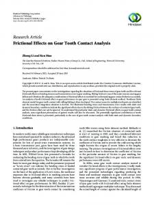
We use the contact patch test to check the ability of node-to-surface contact algorithm to transfer the stresses uniformly through the interface. Figure 3.8 shows the typical contact patch test, which consists of a punch in contact with a rectangular foundation, with a distributed load applied at the top free surfaces of the structure.
Figure 3.8 Contact Patch Test
43 From the equilibrium of the free body A, the applied pressure P must be equal to the internal stress tA as stated in Equation (3.73):
∫ Pd Γ = ∫ t
ΓAtop
A
(3.73)
dΓ
ΓAbottom
Assuming the finite element discretization in element A is complete and can reflect a constant state of pressure, then:
∫ Pd Γ = ∫ Pd Γ
ΓAtop
(3.74)
ΓAbottom
This implies that:
∫t
A
dΓ=
ΓAbottom
∫ Pd Γ
(3.75)
ΓAbottom
The work done by body A on body B is:
∫t
A
A
.u dΓ =
ΓAbottom
∫ P.u
A
dΓ
(3.76)
ΓAbottom
Similarly, the work done by body B on body A is: B
B ∫ t .u dΓ
(3.77)
ΓBtop
For the equilibrium to hold at the interface, the following must be true:
∫
P.u A d Γ =
Γ Abottom
P.u B d Γ
∫
(3.78)
Γ Abottom A
∫ P.u dΓ =
ΓAbottom
B
B ∫ t .u dΓ
(3.79)
ΓBbottom
For the transfer of pressure to be complete, the traction field on ΓBtop = P is: A
A ∫ t .u dΓ =
ΓAbottom
A
∫ P.u dΓ
ΓAbottom
(3.80)
44 Since ΓAbottom = ΓBtop = ΓC , this leads to:
P.u A d Γ =
∫
Γ Abottom
∫
P.u B d Γ = 0
(3.81)
Γ Abottom
Since P is, equation (3.81) implies that, for the pressure transfer to be complete, the following condition has to hold: 1
2
∫ u dΓ − ∫ u dΓ = 0
Γc
(3.82)
Γc
Therefore, for the contact formulation to pass the patch test, the variational field needs to be continuous, at least in a weak sense, across the interface. The node-to-surface contact algorithm does not pass the patch test since the gap function gn guarantees continuity at the slave nodes only.
Figure 3.9 Complete Transfer of Stresses Through the Interface in Conforming Meshes (Left) Versus Incomplete Transfer of Stresses in Non-Conforming Meshes (Right)
The node-to-surface algorithm for NCM does not pass the contact patch test due to the inaccurate transfer of forces from one side to the other. The difference between
45 conforming meshes and NCM is shown in Figure 3.9, which is a demonstration of the patch test using Abaqus. Figure 3.9 (left) shows a complete transfer of stresses along the interface in conforming meshes, while Figure 3.9 (right) shows incomplete transfer of stresses along the interface in non-conforming meshes.
3.3.5
Interface Model: EDGA
We implement the Enriched Discontinuous Galerkin Approach(EDGA)(Haikal, 2009) to solve the continuity problem at the interface of NCMs. The EDGA is a primal approach that enables a two-pass strategy for the enforcement of geometric compatibility along the interface through local enrichment. The method is based on a local enrichment designed to guarantee geometric compatibility at all nodes of the interface, without the need of a master-slave definition. The local enrichment transforms the geometric compatibility condition to a set of node-to-node constraints by inserting a new node where a node meets a surface. This local enrichment can be enforced at all nodes along the interface. Completeness of the finite element interpolation in the enriched element can be preserved by updating the set of Lagrangian shape functions to account for the additional node. Since the displacement between the nodes remains discontinuous, a Discontinuous Galerkin (DG) stabilization is applied to ensure the continuity of the tractions in a weak form along the interface. The EDGA is explained below(Haikal, 2009). We start by discussing the fully coupled (bilateral) case and then move to release tangential displacement constraints to enable sliding along the interface.
46 3.3.5.1 EDGA: The Fully Coupled Case When contact occurs between a node p and the top surface 34 of an element 1234, a node is inserted on the element surface at the location of contact. The following equations define the shape functions of the inserted node 5as illustrated in Figure 3.10
1 (ζ + 1)(ζ 1 − 1) ~ N p (ζ , ζ p ) = (ζ 2 + 1) p1 2 (ζ + 1)(ζ p − 1)
(3.83)
To preserve the interpolatory nature of the finite element basis and its partition of unity property, the shape functions associated with existing nodes are modified as follows:
~ N α = N Qα 4 − N Qα 4 (ζ p ) N p
(3.84)
~ N α (ζ , ζ p ) = N α (ζ ) − N α (ζ p ) N p (ζ , ζ p )
(3.85)
~ ~ where N p (ζ , ζ p ) is the shape function of the enriched node, N Qα 4 is the shape function of
~ Q4 element for α= 1,…, 4, and N α are the modified (enriched) element shape functions.
Figure 3.10 Local Enrichment of the Interface Element for the Following Cases: (a) Single Node, (b) Multiple Nodes, and (c) Added Node Reference in the Parent Domain (Haikal, 2009).
47 The goal of the DG-based stabilization procedure to ensure a complete transfer of the traction field across the interface. To better understand the motivation behind the stabilization approach, we refer to the formulation of the coupled problem described in Section 3.2.1.We can write the Galerkin form of the governing equations in the material coordinates in terms of the First Piola-Kirchhoff stress tensor P as follows:
− ∑ ∫ P.∇ X u dV +∑ ∫ b 0 .u dV +∑ ∫ h 0 .u dΓ +∑ ∫ PN + .u + dA e Ve
e Ve
e Γet
i
Ai+
(3.86)
+ ∑ ∫ PN − .u − dA = 0 i
Ai−
where, b0 is the body force, h0 is the applied traction,
N+ , u+
and
N− , u−
are the
normal and variational displacement vector on each side of interface, and Ai is the interelement interface in the undeformed configuration. It is worth noting that this form of the weak statement of equilibrium and equation (3.2) are exactly equivalent, with the gradient operator defined with respect to the material and spatial coordinates, respectively. As we observed in equation (3.5), it is obvious from Equation (3.86) that, if u is continuous across the element boundaries, the interface term becomes:
∑ ∫ PN i
Ai+
+
.u + dA + ∑ ∫ PN − .u − dA = ∑ ∫ [P + + P − ]N.u dA = 0 i
Ai−
i
(3.87)
Ai−
which weakly enforces the equilibrium of tractions along the element interface. If u is not continuous along the element interfaces, equilibrium of tractions does not necessarily hold, and the interface term could be the cause of numerical instability in the solution. In order to stabilize the solution and enforce traction continuity, the weighted residual of the interface traction equilibrium is included in Equation (3.85) to give:
48
− ∑ ∫ P.∇ X u dV +∑ ∫ b 0 .u dV +∑ ∫ h 0 .u dΓ +∑ ∫ PN + .u + dA e Ve
e Ve
e Γet
i
Ai+
+ ∑ ∫ PN − .u − dA − ∑ ∫ [PN + + PN − ].u h dA = 0 i
i
Ai−
h
(3.88)
Ai−
where, u = (u + u ) / 2 is the average of the variational displacements along the +
−
interface, which guarantees an unbiased method. Simplifying and rearranging the terms in the above equation, gives the following:
− ∑ ∫ P.∇ X u dV +∑ ∫ b 0 .u dV +∑ ∫ h 0 .u dΓ + e Ve
e Ve
e Γet
1 PN + .[ u + − u − ]dA ∑ ∫ 2 i Ai+
1 + ∑ ∫ PN − .[ u − − u + ]dA = 0 2 i Ai−
(3.89)
It should be noted that if u + = u − = u h , the interface terms go to zero and the formulation returns back to the standard continuous Galerkin method. The key differences between the EDGA formulation and standard DG formulations can be summarized as follows (Haikal, 2009): 1. Unlike typical DG formulations where compatibility of displacement holds in a weak sense along the element interfaces, this method relies on a strong enforcement of displacement continuity at the nodes. 2. The traction stabilization terms are based on local estimates of interface tractions, unlike DG formulations that typically employ numerical fluxes with a userdefined stabilization parameter. 3. The formulation is consistent and includes the continuous Galerkin method as a subset. Therefore, it can be easily integrated in a standard Finite Element code.
49 We verify our implementation of the EDGA using the standard contact patch test shown in Figure 3.11.Nodes h, f, g are insterted to transfer the continuity condtion from a node-to-surface to a node-to-nodeconstraint. The stabilization procedure ensures that the formulation passes the patch test within machine precision.
Figure 3.11 Contact Patch Test with EDGA
3.3.5.2 EDGA: Contact with Sliding In sliding cases, the bodies in contact are allowed to move tangentially with respect to each other and the continuity condition applies to the normal component of the displacement only. The objective of the enrichment explained in Section 3.3.5 is to transform the node-to-surface contact constraint to node-to-node. This objective is still valid for the contact problem with sliding. However, as shown in Figure 3.12, the difference is that node p is able to move from the surface if the contact constraint is deactivated. This makes the spatial coordinates of node p and the enriched node r
50 independent quantities. Therefore, node p can separate from the contact element surface, while the enriched node r keeps its coordinates.
Figure 3.12 Enrichment Updating Procedure for Sliding (Haikal, 2009)
In order to update the spatial and material coordinates of the enriched node, the following procedure is applied: r 1. Given the previous enrichment reference ζ , spatial element coordinates
xα
for α = 1 through n, and the spatial location of the contact node
x r and
x p , the
p following equation is solved to find ζ :
x r = N α (ζ p , ζ r )xα + N r (ζ p , ζ r )x r
(3.90)
r* p 2. Assuming that the contact surface ζ j = c, the new enrichment location ζ = ζ r* with ζ j = c.
3. The new spatial and material coordinates are computed as:
~ ~ xα = N α (ζ p , ζ r )xα + N r (ζ p , ζ r )x r
(3.91)
~ ~ ~ Xα = N α (ζ r* , ζ r ) Xα + N r (ζ r* , ζ r ) X r = N α (ζ r* )xα
(3.92)
51
4. Set
xr = xr
*
and
Xr = Xr
5. Update the displacement
*
u = xr − Xr .
6. Reiterate until convergence is reached. Although the contact constraints described above enforce geometric compatibility (in the normal sense) at the interface nodes, the displacement field between the nodes remains discontinuous in both directions; i.e. normal and tangential directions. This leads to incomplete transfer of the traction field across the interface. In order to solve this problem, the stabilized DG formulation is applied to the contact interface resulting in weak continuity of the traction field in the normal direction only. Therefore, the stabilization of the interface in a sliding contact problem can be written as follows: − ∑ ∫ P.∇ X u dV +∑ ∫ b 0 .u dV +∑ ∫ h 0 .u dΓ + e Ve
e Ve
e Γet
1 ∑ (n + .PN + )(n + .[u + − u − ]dA 2 i A∫i+
1 + ∑ ∫ (n − .PN − )(n − .[ u − − u + ]dA = 0 2 i Ai−
(3.93)
where n and N are the normal to the deformed and undeformed configurations, respectively, and A is the set of the contact interfaces. This procedure was applied for the elasticity case by Haikal (Haikal, 2009). In this study, we extend this application to the case of plasticity with no major modifications on the above updating procedure.
52
CHAPTER 4. EXTENSION OF THE EDGA FOR PLASTICITY
In this study, the EDGA developed for the coupling of the NCM is extended to model large-deformation contact problems between bodies with inelastic constitutive behavior. The EDGA is a primal approach that enables a two-pass strategy for the enforcement of geometric compatibility along the interface by inserting a new node at contact locations. This local enrichment can be enforced at all nodes along the interface. The enrichment in the element introduces a higher order in the element shape function associated with the nodes located on that interface. Thus, the order of interpolation has to be increased in the direction where the node is inserted. Solving this problem in hyperelasticity is usually accomplished by increasing the order of the Gauss integration scheme, thereby introducing new integration points. This process, however, could be problematic for the case of inelasticity. For history-dependent materials in which plastic strains are stored and accumulated at the Gauss points after each converged load step, the computational history at the integration points before enrichment must be preserved. Therefore, a progressive integration rule such as the Gauss-Kronrod quadrature can be used alternatively. The Gauss-Kronrod quadrature inherits Gauss point locations and provides an additional set of integration points interlaced between the original Gaussian quadrature. To compute the number and locations of additional Kronrod points required to evaluate a
53 given integral accurately, we begin by computing an estimate of the integral with the original Gauss quadrature. Then, we re-compute it using two sets of points combined; the original Gauss points set and Gauss-Kronrod set. The difference between the values of the two sets gives an estimate of the error in the results. The derivation of the GaussKronrod formula is similar to standard Gauss quadrature. The Gauss-Kronrod quadrature and its implementation for the purpose of this research are explained through the following example. Consider the enriched element shown in Figure 4.1. We assume an enrichment of the top surface ζ2 = 1,which introduces a quadratic term inζ1 in the element shape functions associated with the nodes located on this interface, while the order of interpolation with respect to ζ2 remains the same. Therefore, for the element to be integrated properly, the integration rule order has to be increased in the direction of ζ1. For the use of this element in contact simulations, two different sets of GaussKronrod integration points are needed. The first set of points is used inside the element as illustrated in Figure 4.1, where the stresses and plastic strains are computed to find the internal forces and the stiffness of the element. In addition, Gauss-Kronrod integration points are needed on the interface as illustrated in Figure 4.2, to be used for the stabilization terms, where the stresses and plastic strain are computed.
54
Figure 4.1 Q4 Element with Gauss Quadrature Integration Points Inside (Left) and the Enriched Element with Gauss-Kronrod Integration Points (Right)
Figure 4.2 Q4 Element with Gauss Quadrature Integration Points at the Interface (Left) and the Enriched Element with Gauss-Kronrod Integration Points (Right)
Computing the Gauss-Kronrod integration points and weights involves the following steps: •
Evaluating the integral using a N-point Gauss quadrature according to the following equation:
55 1
∫
−1
N
f (x)dx =∑ wk f (x k )
(4.1)
k =1
where wkandxkare the locations and the weights of the original Gauss points. • Evaluating the integral again using a 2N+1Gauss-Kronrod quadrature. The location of the N points from step one is reused. The locations and corresponding weights of N+1additionalpoints are recalculated, as well as the weights associated with the N Gauss points: 1
∫
−1
N
N +1
k =1
j =1
f (x)dx =∑ z k f (x k ) + ∑ m j f (y j )
(4.2)
The set of nodes xk is precisely the one used in the original Gauss quadrature. All the other 3N+2 parameters zk, mj, and yj are chosen such that Equation (3.90) reaches its maximum degree of accuracy. Table 4.1 lists the values of the locations and weights for the Gauss-Kronrod integration points i including the Gauss quadrature for exact integration of a cubic function N=2.
Table 4.1Gauss-Kronrod Quadrature Locations and Weights for N=2 i
Kronrodξ1
Kronrodξ2
Kronrod wi
Gauss wi
1
-0.92582009977
0.57735026918
0.19797979798 ---
2
-0.57735026918
0.57735026918
0.49090909090 1
3
0
0.57735026918
0.62222222222 ---
4
0.57735026918
0.57735026918
0.49090909090 1
5
0.92582009977
0.57735026918
0.19797979798 ---
56 The values of plastic variables at original Gauss points are preserved throughout the analysis. When the enrichment happens and Gauss-Kronrod integration points are added, we propose to compute the values of the plastic variables at the new integration points by interpolation/extrapolation from the existing values using the element shape functions.
57
CHAPTER 5. FRICTIONAL CONTACT
5.1
Frictional Contact Formulation
Frictional contact behavior governs the relationship between tangential interface tractions and the relative tangential motion between two contacting points at the contact interface between the two bodies. We compute the tangential component of the displacement on the interface as u T = [1 − n ⊗ n].(x − x p ) , where [1 − n ⊗ n] is the projection tensor P. Similarly, the tangential component of the gap function, denoting the lateral relative motion between two points across the contact interface is: gT=Pg and the tangential component of the traction vector tat the interface is: tT = Pt. The widely used Coulomb constitutive model is chosen in the present formulation of the frictional contact. According to this model, points along the contact interface can be in either a stick or slip state. The stick state occurs when the tangential component of the interface traction vector, tT, is less than the frictional resistance of the interface, defined to be equal to the normal contact force multiplied by the friction coefficient. In this case, no relative tangential displacement occurs. Slip happens when the applied force reaches the maximum frictional resistance and causes a relative tangential displacement. The stick/slip criterion of the Coulomb model provides can be expressed as an inequality slip function that relates tT and the normal component of the traction tn through the friction coefficient µ as:
58
f (t n , t T ) = t T − µ t n ≤ 0
(5.1)
The stick state occurs when tT ≤ µ and tn, ≥while the slip state occurs when tT >µ tn. This leads to the Kuhn-Tucker conditions for frictional contact:
u T ≥ 0, f ≤ 0, and u T f = 0
(5.2)
To develop the finite element formulation of the frictional contact problem, we start with the virtual work statement. To maintain equilibrium in frictional contact cases, the virtual work functional must include a new term that accounts for the work done by tangential forces at contact locations as follows:
G(u, u , λ ) = ∫ S : Edv − ∫ b : u dv − ∫ t : udΓt + ∫ λgdΓc +GCT (u, u )
(5.3)
GCT (u, u ) = ∫ t T u T d Γc
(5.4)
v
v
Γt
Γc
Γc
where GCT (u, u) is the tangential virtual work at the contact locations. In the case of stick, the work done by the tangential forces vanishes, and therefore, the formulation remains conservative. When slip is detected, the negative work done by the tangential forces leads to a dissipation of energy.
The distinction between stick/slip conditions is required to properly account for the tangential work done on the interface. In the case of stick, a constraint has to be placed on lateral displacements to prevent sliding, whereas in the case of slip, the tangential displacements are released and a tangential force is applied instead.
59 5.2
Enforcing Frictional Contact Constraints
In this thesis, the EDGA formulation is extended for frictional contact; i.e. bodies are allowed to slide tangentially, and the contact constraint is enforced only on the normal direction. Additional terms accounting for the tangential force at the interface are introduced. The Coulomb friction model is selected to represent the constitutive relation at the interface. The moving enrichment is implemented in order to maintain the continuity in the normal direction and the effect of friction is considered for the stick and slip conditions. The Coulomb model indicates no displacement in the case of stick condition, therefore, a zero-lateral displacement condition has to be added to the normal non-penetration constraint for the case of stick. This condition needs to be relaxed if the contact is deemed to result in slip. As discussed in Section 3.3.3, Lagrange multipliers are used to add constraints to the weak form of equilibrium for bodies in contact, as shown in Equations (3.69) and (3.70). In the case of stick, these multipliers correspond to the normal and tangential contact stresses λ N and λT , respectively, that represent the normal and tangential components of the contact traction, respectively. Therefore Equation (3.69) can be rewritten as follows: n
π c (u, λ ) = ∑ (λ N g N + λ T g T )
(5.5)
i =1
When enforcing the normal constraint only in the case of frictionless contact, the above equation will only show the normal term without the tangential as follows:
π c (u, λ ) = π (u) + λg n
(5.6)
60 In order to solve the system of equations for the coupled problem stated in Equation (3.71), the derivative of the gap function with respect to the displacement will only contain the terms associated with the normal component of the gap function gn as follows: T ⎡ ⎛ dg N ⎞ ⎤ G ⎜ ⎟ ⎥ ⎡d ⎤ ⎡f ⎢ K d u ⎝ ⎠ ⎥ ⎢ ⎢ ⎥ = ⎢ ⎢⎛ dg N ⎞ ⎥ ⎣λ N ⎦ ⎢⎣0 0 ⎥ ⎢⎜ du ⎟ ⎠ ⎣⎝ ⎦
⎤ ⎥ ⎥⎦
(5.7)
The above system of equations is solved for the nodal displacements d and the Lagrange multipliers that represent the normal component of the contact pressure only. Methods used in the literature to enforce the contact constraints in frictional cases require a-priori knowledge of whether a point is in stick or slip state. For each increment an assumption of stick /slip condition is made at each contact point. This assumption is checked after completing the solution of the nonlinear problem, typically using the Newton method. If the initial assumption is found to be no longer correct, the Newton solution is repeated under revised assumptions. In a large finite element mesh where the contact state at a number of interface nodes could potentially change between stick and slip, this approach in enforcing frictional constraints has been found to be the source of algorithmic instability. The dilemma in deciding the stick/slip conditions at contact nodes recalls a similar issue in computing stresses in the theory of plasticity. Much like the frictional case, the stresses in plasticity are bound by a “yield” function upon which the material starts accruing irreversible plastic flow that occurs normal to the yield surface and does
61 not correspond to an increase in stress. For frictional contact, tangential slip can be thought of as the equivalent of plastic strain, i.e. an irreversible state of deformation that does not cause an increase in the corresponding stress/force beyond a limit dictated by the yield function of the Coulomb model (Equation 5.1). Furthermore, the stresses and deformations beyond “yielding” in frictional contact are governed by a similar set of Kuhn-Tucker conditions. Therefore, an alternative approach to enforcing frictional contact conditions is to compute the tangential tractions through an inner-subroutine, activated at the contact point, that releases the flow of slip displacement in the case where the yield potential, in this case called the slip criterion, is exceeded assuming stick conditions. This approach is algorithmically superior since it does not require the repetition of the Newton solution anytime the slip criterion is violated and slip is activated at a given contact location, thereby substantially reducing computational cost and potential instability. This method has been adopted by numerous researchers in the frictional contact community (Laursen and Simo, 1993b, Sheng et al., 2006, and Masud et al., 2012) although its application has been restricted to the case of linear elasticity for reasons that will become obvious in the discussion below. The aim of this work is, therefore, to overcome the difficulties of applying this approach to large-deformation problems.
5.3
Plasticity-Inspired Approach
We propose a new plasticity-inspired formulation for hyperelastic largedeformation frictional contact. This approach handles the numerical issues encountered when modeling the stick/slip Coulomb frictional contact models. Our approach handles
62 the stick/slip condition in an inner loop inside the Newton solver without the need of a repeated solution. We start our formulation for the case of small deformations, which has been done also in other studies in literature, in order to illustrate the challenge in extending this approach to the large-deformation frictional contact problem.
5.3.1
Small Deformation Frictional Contact
The plastic tangential slip is governed by a constitutive equation that can be derived using the standard concepts of the elasto-plasticity. For small deformations, the total displacement is decomposed into elastic and plastic parts: u = u e + u p . Note that, due to the linearity of the problem, the decomposition of the displacement field yields to a similar decomposition of the traction field: e
p
𝒕 𝒖 = 𝐊𝒖 = 𝐊 𝒖! + 𝒖! = 𝐊𝒖! + 𝐊𝒖! or t (u) = t (u ) + t (u )
(5.8)
As shown in equation (5.1), the slip criterion can be expressed as follows:
f = t n+1 .P 2 t n+1 − µ t n ≤ 0
(5.9)
The value of f ≤ 0 indicates a stick state; while f > 0 is an inadmissible state that indicates the occurrence of tangential slip. Therefore, the return mapping that was illustrated previously in Figure 3.4 is performed in order to return the trial tractions
t trial n+1
to the slip surface. We assume that the “flow” of irreversible slip displacement occurs tangent to the surface, a direction that corresponds to associative flow in the direction of the normal to the yield surface r, which is computed as follows:
r=
Pt t .P 2 t
(5.10)
63 The variable γ takes the slip criterion back to the yield surface, i.e. f = 0 . To calculate γ, the nonlinear system of equations is solved using Newton’s method as follows:
f = t n+1 .P 2 t n+1 − µ t n+1n
∂f = ∂γ
∂γ =
t n +1 P 2
t n +1 ∂γ
t n +1 n ∂γ
(5.12)
value of γ ⎯update ⎯⎯the⎯ ⎯⎯→ γ = γ − ∂γ
(5.13)
t n +1 .P 2 t n +1
f ∂f ∂γ
(5.11)
+µ
The tangential tractions at the interface in the case of a linear material model are computed using the following incremental expression, based on the Backward Euler (virtual) time integration scheme, where the subscripts denote the updated quantities at step n + 1 : trial t trial + K (u n +1 − u np ) n +1 = t n
(5.14)
t n+1 = t trial − γ K rn+1 n +1
(5.15)
∂t n +1 = −K rn +1 ∂γ
(5.16)
u p = u p + γ rn+1
(5.17)
The friction force is history-dependent, therefore the plastic displacement is computed for every converged step to be considered in the next step as: u p = u p + γ rn+1 .
64 Consistent Tangent: The tangent matrix T is computed by evaluating the partial derivative of the traction with respect to the displacement as follows:
T=
∂t n+1 ∂r ∂γ = K − γ K n+1 − K rn+1 ∂u n+1 ∂u n+1 ∂u n+1
(5.18)
In order to compute the tangent T, the partial derivative of the slip function with respect to the displacement is used as follows:
∂f ∂t ∂f = n+1 n+1 = 0 ∂u n+1 ∂t n+1 ∂u n+1
(5.19)
P 2 t n+1 ∂f = +µn ∂t n+1 t n+1 .P 2 t n+1
(5.20)
The partial derivative of the direction vector with respect to the displacement is computed as follows:
∂rn+1 ∂rn+1 ∂t n+1 = ∂u n+1 ∂t n+1 ∂u n+1
(5.21)
∂rn +1 [P − rn +1 ⊗ P rn +1 ] = =S ∂t n +1 t n +1 .P 2 t n +1
(5.22)
The partial derivative of γ with respect to the displacement is computed from Equation (3.109) as follows:
h T K[I − γ Srn +1 ] ∂γ = ∂u n +1 h T Kr
(5.23)
Substituting the previous derivatives into Equation (5.15), and rearranging the terms using w and v, we find:
65
T=
where, v =
K −ν⊗w [I + γ (K − ν ⊗ w )S] Krn +1 h T Kr
and w =
Kh h T Kr
(5.24)
.
It is worth noting that, without additional consideration, this formulation does not guarantee a perfect stick condition. In other words, there could exist a non-zero value of lateral displacement that would not cause the violation of the slip criterion. This issue, however, can be remedied by enforcing an additional constraint on the tangential component of the “stick” displacement to be zero.
5.3.2
Large-Deformation Frictional Contact
Extending the above to the case of large-deformation problems is hindered by the fact that equation 5.8 no longer holds when the traction is a nonlinear function of the displacements. In other words, an additive decomposition of the displacement field does not translate into a similar result for the traction field. Therefore, the return-mapping algorithm, as described above cannot be implemented. Our first attempted approach remedy this problem was to follow a procedure similar to large-deformation computational plasticity theory by following the idea of a multiplicative decomposition of the deformation gradient into elastic and plastic parts as: F = F e F p (Section 3.2.5.2). For the case of frictional contact, the elastic and plastic parts of F would correspond to the stick and slip modes of response, respectively. The derivation follows exactly the same steps as computational plasticity by computing the strain be and stretches λe as derived in Equations (3.33) and (3.44).
66 −1
The fact that the plastic deformation is computed through the strain tensor CP , however, as shown previously in Equation (3.46), limits the application of this approach for frictional contact since it would not be possible to enforce perfect stick conditions. This is due to the fact that the plastic displacement up required to enforce these conditions is not a variable in this formulation. The second attempted approach was based on the observation that enforcing perfect stick conditions strictly requires an additive split of the displacement field:
u = u e + u p , as is done for the case of small deformations. To circumvent the fact that this decomposition does not correspond to an additive split of the traction field, we propose using a linearized form of the traction vector, based on a Taylor series expansion around the elastic (stick) displacement as follows:
t (u) = t(u e ) − ∇t u p
(5.25)
The tractions associated with the stick component of the displacement can be computed as follows, regardless of whether the total traction t(u) results in a final stick or slip condition:
𝐭 𝒖! = 𝐭 𝒖 − 𝐊 𝒖! 𝒖!
(5.26)
where K is the instantaneous tangent tensor. When discretized using the Backward Euler scheme, Equation (5.26) becomes: !
!
𝐭 !!! 𝒖!!!! = 𝐭 𝒖!!! − 𝐊 𝒖!!!! 𝒖!!! = 𝐭 𝒖!!! − 𝐊 𝒖!!!! 𝒖! + ! 𝛾𝒓!!! = 𝐭 !"#$% !!! 𝒖!!! − 𝛾𝐊 𝒖!!! 𝒓!!!
with the trial tractions computed as follows:
(5.27)
67
t trial n +1 (u) = t n +1 (u n +1 ) − K u n
(5.28)
Note that the first term in this equation involves computing the traction vector using a hyperelastic law. The slip criterion is then computed and the tractions are updated in the same manner as the small deformation case; Equation (5.15). The plastic displacement is stored and updated as in Equation(5.17). For each load increment the total displacement P
is updated as: u = u-u . It is useful to point out that this formulation assumes that the amount of plastic slip within a given load step is small enough for the Taylor series expansion to hold. In the case of large slip, this assumption can be satisfied using appropriately small load increments. When slip is persistent over a large number of load steps, the large total slip should be of no consequences since the value of the tangential traction should remain relatively constant as it is bounded by the slip criterion.
68
CHAPTER 6. NUMERICAL RESULTS
In this chapter, we demonstrate the accuracy and efficiency of the proposed formulation for inelastic contact and friction in the presence of large deformations. We start by verifying our implementation of the Gauss-Kronrod quadrature integration scheme using a simple example involving a single Q4 element with enrichment under uniaxial compression. Next, we verify our implementation of the EDGA for elasticity using the contact patch test within the constraints of linear elasticity and small deformations. We then move to the case of large deformations and show results for the contact patch test using both linear and nonlinear material laws with plasticity. The cases are analyzed first without applying the EDGA, and then repeated with the proposed EDGA formulation for plasticity. Next, the formulation is extended to consider the friction for both stick and slip conditions; Coulomb friction model was selected to represent the constitutive relation at the interface. The sliding contact patch test was then performed for the cases of hyperelasticity and plasticity. Finally, case studies are presented to verify the effectiveness of the proposed approach for handling Coulomb friction conditions, for the cases of small and large deformations, and we demonstrate enhanced performance compared with ABAQUS.
69 6.1
Verification of the Gauss-Kronrod Integration Scheme
We use a single Q4 element under uniaxial tension for the verification of the Gauss-Kronrod Integration scheme. The Q4 element shown Figure 4.1 has an elastic modulus (E) =30,000 ksi, Poisson’s ratio (υ) = 0.3, and yield stress (fy) = 60 ksi. We assume plain-strain conditions. The applied distributed load P is equal to 65 ksi. This setup is identical to the well-known patch test using finite elements and the expected solution is a constant pressure profile in the element. This element is enriched at the bottom surface, which introduces a higher order term in the element shape functions associated with the enriched node. The Gauss-Kronrod quadrature integration points are used along the enriched side as shown in Figure 6.1. The results in Figure 6.2 show that the Q4 element with Gauss-Kronrod quadrature integration points passes the patch test and reflects a constant stress distribution exactly. Figure 6.3 shows the Q4 element deformed shape, which is also consistent with the exact solution.
Figure 6.1 Patch Test for Q4 Element with Enrichment (Left) and the Gauss-Kronrod Quadrature Integration Points in the Parent Element (Right)
70
Figure 6.2 Stress Distributions for Q4 Element with Gauss-Kronrod Integration Points
Deformed Configuration(Magnification =1000) 0.5 0.45 0.4 0.35 0.3
4
3
0.25 0.2
1
0.15 0.1 0.05 0
1
0
0.1
0.2
0.3
0.4
0.5
2
Figure 6.3 Deformed Shape for Q4 Element with Gauss-Kronrod Integration Points
71 6.2
6.2.1
Contact Patch Test
Small Deformation Linear Elastic Case
We consider the contact patch test configuration of Figure 3.7 and assume small deformations and a linear elastic material with E = 30,000ksiand υ = 0.3. A distributed load of P = 200 ksi is applied on the top free surfaces of both bodies. The domains are discretized using Q4 elements under plane strain conditions. This case serves the purpose of verifying our implementation of the EDGA, showcasing its superiority in handling interface tractions when compared to the standard bode-to-surface formulation. Figures 6.4 (left) and 6.5 (left) show the deformed shape and stress distributions, respectively, obtained with a standard node-to-surface contact formulation without treating the non-conforming interface. The results show an incomplete transfer of the traction along the interface and inaccurate deformed shape. Figures 6.4 (right) and 6.5 (right) show the solution obtained by applying the EDGA at the interface. The results show that the deformed configuration and the stress distributions reflect a state of constant pressure up to machine precision.
72 Deformed Configuration(Magnification =10)
Deformed Configuration(Magnification =10)
1
1
4
0.9
3
4
0.9
3
0.8
0.8
0.7
0.7
1
1 0.6
0.6 0.5
1 11
10
0.5
2 12
9 13
8
0.3
2
1 11
0.3
3
0.2
0.2
0.1
0.1
0
10
9 13
2 12
8
0.4
0.4
5 0
0.2
0.4
6
0.6
0.8
7
1
0
2
5
0
0.2
3
0.4
6
0.6
0.8
1
7
Figure 6.4 Contact Patch Test for the Small Deformation Linear Elastic Case: Deformed Shape without EDGA (Left) and with EDGA (Right)
Figure 6.5 Contact Patch Test for the Small Deformation Linear Elastic Case: Stress Field without EDGA (Left) and with EDGA (Right)
73 6.2.2
Material and Geometric Nonlinearity
We repeat the solution to the above problem under the conditions of material and geometric nonlinearity. In this case, the problem deviates from the standard patch test with a known exact solution. However, we expect the effects of nonlinearity on the deformed shape to be minimal so that the results would still be in the neighborhood of those obtained for the linear case, especially since, by virtue of equilibrium, we can expect that the solution to reflect a state of constant pressure in the normal direction. These results serve to demonstrate the effectiveness of our implementation of the large deformations formulation as well as the nonlinear material laws.
6.2.2.1 Large-Deformations, Linear Elastic Material In this case, we investigate the effects of large deformations assuming a linear elastic material with E = 30,000ksiand υ = 0.3. A distributed load of P = 100 ksi is applied on the top free surfaces of both bodies. The domains are discretized using Q4 elements under plane strain conditions. Figures 6.6 (left) and 6.7 (left) show the solution obtained with a standard node-to-surface contact formulation without treating the nonconforming interface. The results show an incomplete transfer of the traction along the interface and the deformed shape is not logical since the applied pressure is uniform and, accordingly, nodes 8, 9, and 10 are expected to displace similarly in the vertical direction. Figures 6.6 (right) and 6.7 (right) show the solution obtained by applying the EDGA at the interface. The results show that the deformed configuration and the stress distributions reflect a state of constant pressure up to machine precision.
74
Deformed Configuration(Magnification =1000)
Deformed Configuration(Magnification =1000)
1
1
4
0.9
3
0.8
3
0.8
0.7
0.7
1
0.6
1 11
10
1
0.6
0.5
0.5
2 12
9 13
10
8
0.4
1 11
9 13
2 12
8
0.4
0.3
2
0.3
3
0.2
2
3
0.2
0.1 0
4
0.9
0.1
5
0
0.2
0.4
6
0.6
0.8
1
7
0
5
0
0.2
0.4
6
0.6
0.8
1
7
Figure 6.6 Contact Patch Test for the Linear Elastic Case: Deformed Shape without EDGA (Left) and with EDGA (Right)
Figure 6.7 Contact Patch Test for the Linear Elastic Case: Stress Field without EDGA (Left) and with EDGA (Right)
75 6.2.2.2 Large Deformations with Hyperelasticity In this case, we assume a hyperelastic material with the properties E = 30,000ksi and υ = 0.3. A distributed load of P = 1000ksi is applied to the top free surfaces of both bodies. The domains are discretized using Q4 elements under plane strain conditions. Figures 6.8 (left) and 6.9 (left) show the solution obtained using the standard node-tosurface interface formulation without treating the non-conforming interface. Similar to the previous case, the results show an incomplete transfer of tractions along the interface and the deformed shape does not make sense since the applied pressure is uniform and accordingly nodes 8, 9, and 10 are expected to deform similarly. Figures 6.8 (right) and 6.9 (right) show the solution obtained by applying the EDGA at the interface. The results show that the deformed configuration and the stress distributions pass the patch test up to machine precision, which is also similar to the previous case.
Deformed Configuration(Magnification =10)
Deformed Configuration(Magnification =10)
1
1
0.9
0.9
0.8
4
4
3
0.8
3
0.7
0.7 1
0.6
0.6 1
0.5
0.5
10 0.4
1 11
10
2 12
9 13
8
0.3
0.3 2
0.2
3
9 13
2 12
8
2
3
0.2
0.1 0
1 11
0.4
0.1 5
0
0.2
0.4
6
0.6
0.8
1
7
0
5
0
0.2
0.4
6
0.6
0.8
1
7
Figure 6.8 Contact Patch Test for the Nonlinear Elastic Case: Deformed Shape without EDGA (Left) and with EDGA (Right)
76
Figure 6.9 Contact Patch Test for the Nonlinear Elastic Case: Stress Field without EDGA (Left) and with EDGA (Right)
6.2.2.3 Large-Deformation with Von Mises Plasticity In this case, an elasto-plastic material with the Von Mises yield criterion is used with E = 30,000 ksi, υ = 0.3, and fy = 60 ksi. A distributed load of P = 70 ksi is applied to the top free surfaces of both bodies. The domains are discretized using Q4 elements under plane strain conditions. Figures 6.10 (left) and 6.11 (left) show the solution obtained without treating the non-conforming interface. The results show inaccurate pressure distribution and the deformed shape displays similar inaccuracies at nodes 8, 9, and 10. Plasticity in this problem is activated, since the applied load is greater than fy. The plastic strain at the integration points is around 0.00965. Figures 6.10 (right) and 6.11 (right) show the solution obtained by applying the EDGA for plasticity using GaussKronrod quadrature integration points inside the element to find the tangent and the
77 internal forces and at the interface for the stabilization terms. As obtained in the previous two cases, the results of this case show that the deformed configuration and the stress distributions pass the patch test up to machine precision.
Deformed Configuration(Magnification =100)
Deformed Configuration(Magnification =100) 1
1 4
4
3
0.9
0.9
0.8
0.8
3
0.7
0.7
1
1 0.6
0.6 0.5
1 11
10
0.5
2 12
9 13
8
0.3
2
1 11
0.3
3
0.2
0.2
0.1
0.1
0
10
9 13
2 12
8
0.4
0.4
5 0
0.2
0.4
6
0.6
0.8
1
7
0
2
5 0
0.2
3
0.4
6
0.6
0.8
1
7
Figure 6.10 Contact Patch Test for the Elasto-Plastic Case (Von Mises): Deformed Shape without EDGA (Left) and with EDGA the Extension for Plasticity (Right)
Figure 6.11 Contact Patch Test for the Elasto-Plastic Case (Von Mises): Stress Field without EDGA (Left) and with EDGA and the Extension for Plasticity (Right)
78 In this case, the patch test is also performed in a different configuration as shown in Figure 6.12 to show that the Gauss-Kronrod quadrature is able to handle elements with non-constant Jacobian. An elasto-plastic material with the Von Mises yield criterion is used with E = 30,000 ksi, υ = 0.3, and fy = 50 ksi. A distributed load of P = 60 ksi is applied to the top free surfaces of both bodies. The domains are discretized using Q4 elements under plane strain conditions. Figures 6.13 (left) and 6.13 (left) show the solution obtained without treating the non-conforming interface. The results show inaccurate pressure distribution and the deformed shape is again inconsistent with the result expected with constant pressure. Plasticity in this problem is again activated, since the applied load is greater than fy. The plastic strain at the integration points is around 0.00895. Figures 6.13 (left) and 6.13 (right) show the solution obtained by applying the EDGA for plasticity using Gauss-Kronrod quadrature integration points inside the element to find the tangent and the internal forces and at the interface for the stabilization terms. As obtained in the previous two cases, the results of this case show that the deformed configuration and the stress distributions pass the patch test up to machine precision.
79
Figure 6.12 Contact Patch Test for the Elasto-Plastic Case (Von Mises)
Figure 6.13 Contact Patch Test for the Elasto-Plastic Case (Von Mises): Stress Field without EDGA (Left) and with EDGA and the Extension for Plasticity (Right)
80 6.2.2.4 Large-Deformation with Drucker-Prager Plasticity In this case, an elasto-plastic (Drucker-Prager) material is used with E = 30,000 ksi, υ = 0.3, cohesion (c) = 10 ksi, friction angle (φ) = 35o, and dilation angle (ά) = 10o. A distributed load of P = 90 ksi is applied to the top free surfaces of both bodies. The domains are discretized using Q4 elements under plane strain conditions. Figures 6.14 (left) and 6.15 (left) show the solution obtained without applying the EDGA with plasticity at the interface. The results show inaccurate pressure distributions and the deformed shape shows obvious errors at the locations of nodes 8, 9, and 10. Plasticity in this problem is activated, and the yield function is computed at each integration point with f(σ,εp)>0. The plastic strain at the integration points is around 0.00497. Figures 6.14 (right) and 6.15 (right) show the solution obtained by treating the interface by EDGA and its extension for the plasticity. As obtained in the previous case, the results of this case show that the deformed configuration and the stress distributions pass the patch test up to machine precision.
Deformed Configuration(Magnification =100)
Deformed Configuration(Magnification =100) 1
1 4
4
3
0.9
0.9
0.8
0.8
3
0.7
0.7
1
1 0.6
0.6 0.5
1 11
10
0.5
2 12
9 13
8
0.3
2
1 11
0.3
3
0.2
0.2
0.1
0.1
0
10
9 13
2 12
8
0.4
0.4
5 0
0.2
0.4
6
0.6
0.8
1
7
0
2
5 0
0.2
3
0.4
6
0.6
0.8
1
7
Figure 6.14 Contact Patch Test for Elasto-Plastic Case (Drucker-Prager): Deformed Shape without EDGA (Left) and with EDGA and the Extension for Plasticity (Right)
81
Figure 6.15 Contact Patch Test for Elasto-Plastic Case (Drucker-Prager): Stress Field without EDGA (Left) and with EDGA and the Extension for Plasticity (Right)
6.3
Sliding Patch Test
Figure 6.16 shows the sliding patch test where a horizontal displacement u is applied to the punch causing it to slide along the foundation surface. The sliding patch test is performed for two cases: hyperelasticity and Von Mises plasticity.
Figure 6.16 Sliding Patch Test
82 6.3.1
Sliding Patch Test for Hyperelasticity
This example is used to show the ability of the formulation to handle a moving enrichment due to sliding. In this case, the interface between the top and the foundation is assumed to be totally frictionless with no resistance to relative sliding. A hyperelastic material is used with the properties E = 30,000ksi and υ = 0.3. A horizontal displacement u=0.03 is applied to the punch and a distributed load of P = 1000ksi is applied to the top free surfaces of both bodies. The domains are discretized using Q4 elements under plane strain conditions. Figures 6.17 (left) and 6.18 (left) show the solution obtained using the standard node-to-surface interface formulation without treating the non-conforming interface. The results show an incomplete transfer of traction along the interface and the deformed shape is not accurate. Figures 6.17 (right) and 6.18 (right) show the solution obtained by applying the EDGA at the interface. The results show that the deformed configuration as expected and the stress distributions pass the patch test in the normal direction up to machine precision.
Figure 6.17 Sliding Patch Test for the Nonlinear Elastic Case: Deformed Shape without EDGA (Left) and with EDGA (Right)
83
Figure 6.18 Sliding Patch Test for the Nonlinear Elastic Case: Stress Field without EDGA (Left) and with EDGA (Right)
6.3.2
Sliding Patch Test for Von Mises Plasticity
In this case, an elasto-plastic material with Von Mises yield criterion is used with the properties E = 30,000ksi, υ = 0.3, and fy = 60 ksi. A horizontal displacement u = 0.03 is applied and a distributed load of P = 70 ksi is applied to the top free surfaces of both bodies. The domains are discretized using Q4 elements under plane strain conditions. Figures 6.19 (left) and 6.20 (left) show the solution obtained using the standard node-tosurface interface formulation without treating the non-conforming interface. The results show an incomplete transfer of traction along the interface and the deformed shows obvious errors on the interface. Figures 6.19 (right) and 6.20 (right) show the solution obtained by applying the EDGA at the interface. The results show that the deformed configuration is accurate and the stress distributions pass the patch test in the normal direction up to machine precision.
84
Figure 6.19 Sliding Patch Test for Von Mises Plasticity Case: Deformed Shape without EDGA (Left) and with the Extension of the EDGA (Right)
Figure 6.20 Sliding Patch Test for Von Mises Plasticity Case: Stress Field without EDGA (Left) and with the Extension of the EDGA (Right)
85 6.4
Numerical Examples for Friction
In this section we show a number of numerical examples to demonstrate the effectiveness and capability of the proposed frictional interface formulation for largedeformation contact problems. In these examples, we will omit units in input parameters and assume consistent inputs. For example, if the modulus of elasticity is interpreted to be in ksi, all resulting stresses will be in ksi and displacements will accordingly be in inches. If units are assumed to be consistent, the particular choice of these units are otherwise of no influence on the numerical values of the results.
Numerical Example 1 The first example represents a simple configuration of the punch and the foundation used in the sliding patch tests as shown in Figure 6.16. The two domains have the same modulus of elasticity of 30,000 and Poisson’s ration of 0.3. A vertical pressure P =200 and a prescribed horizontal displacement u = 0.04 are applied as shown in Figure 6.16. The vertical and horizontal loadings were applied in nine increments, assuming large deformations. Coulomb frictional coefficient of 0.4 is used. The proposed plasticityinspired formulation is applied to the interface. Figure 6.21shows the deformed shapes at each load increment. The results show that node 1 (bottom left corner of Body A) is slipping while node 2 (bottom right corner of Body A) is sticking along the interface. This proves the capability of the proposed frictional interface formulation in handling both the stick and slip conditions.
86
Figure 6.21Incremental Deformation for Numerical Example 1
Numerical Example 2 The second numerical example is obtained from Simo and Laursen (1992) and is used to verify the implementation of the plasticity-inspired framework for friction for the case of linear elasticity wz small deformations. The example considers an elastic block pulled against a rigid foundation resulting in lateral sliding. To minimize code modification, we replaced the rigid foundation with solid elements having a very high modulus of elasticity of 10000 and Poisson’s ratio of 0.0. A Coulomb friction coefficient of 0.5 is used on the block-foundation interface. The block has an elastic modulus of
87 1000 and Poisson’s ratio of 0.3. To follow the exact conditions used by the authors in this paper, no frictional stress is allowed to develop at the first and last nodes of the contact surface due to the uplifting at the edges. Therefore, these ends are assumed not to be in contact with the foundation. The elastic block is subjected to a vertical and horizontal loading as shown in Figure 6.22. The resulting deformed shape shown in Figure 6.23 reveals that our formulation reflects the expected deformed shape in which the block deformed vertically under the normal loading and pulled to the right as a result of the horizontal load. The deformation shape also confirms the assumption of uplift at the corner nodes and is identical to the one reported in the reference. Figure 6.24 and 6.25 show the distribution of vertical and horizontal stresses in the elastic block and foundation, and display higher stress values along the edges closest to the applied loads. It is useful to point out that mesh refinement was not considered in this study in order to produce results comparable with those reported by Simo and Laursen using the mesh shown in Figure 6.22.
Figure 6.22 Geometry and Loading Conditions for Numerical Example 2
88 Deformed Configuration(Magnification =4) 1.5
1
0.5
0
-0.5
-1
-1.5 -2
-1.5
-1
-0.5
0
0.5
1
1.5
2
Figure 6.23 Deformed Shape for Numerical Example 2
Stresses Sxx - NOT averaged 60 40 1
20 0
0.5
-20 0
-40 -60
-0.5
-80 -100
-1
-120 -1.5
-140 -1.5
-1
-0.5
0
0.5
1
1.5
2
Figure 6.24 Horizontal Stress Distribution for Numerical Example 2
The distribution of interface stresses is shown in Figure 6.24. For a consistent comparison with the results of Simo and Laursen, these stresses were computed from the nodal tractions vector, normalized by the element length. Both the normal and tangential tractions show perfect agreement.
89 Stresses Syy - NOT averaged
1
-50
0.5
-100
0 -150 -0.5 -200 -1 -250 -1.5 -2
-1.5
-1
-0.5
0
0.5
1
1.5
2
Figure 6.25 Normal Stress Distribution for Numerical Example 2
Normal Stress - Our Approach
300
Tangential Stress - Our Approach
250
Normal Stress - Simo and Laursen, 1992 Tangential Stress - Simo and Laursen, 1992
Stress at the Interface
200 150 100 50 0 -50
0
1
2
3
4
-100 -150
Figure 6.26 Tangential and Normal Stresses along the Interface for Numerical Example 2
90 Numerical Example 3 This numerical example simulates the contact between two hyperelastic bodies with the configuration shown in Figure 6.25, where the lengths AC = CE = EF = FA = IH = JG =3, and IJ = HG = 9. Bodies 1 and 2 are hyperelastic; body 1 is subjected to a normal pressure of 90 and a prescribed displacement u = 5. Coulomb friction coefficient of 0.4 is used. Body1 and body 2 has an elastic modulus of elasticity of 3000 and 10000 respectively, and Poisson’s ratio of 0.3 and 0.0, respectively. The solution was obtained using our formulation approach and ABAQUS. The resulting deformed shape shown in Figure 6.28 reveals that our formulation reflects a logical deformed configuration in which body 1 deformed vertically under the normal loading and pulled to the right as a result of the horizontal load. Figures 6.29 and 6.30 show the distributions of the resulting horizontal and normal stresses in bodies 1 and 2. The stress values are higher at locations closest to the applied loads with an excellent match between ABAQUS and our formulation results. The ABAQUS contact formulation used the Penalty method to enforce the contact constraints. It is noteworthy to mention that it was hard for ABAQUS to converge for this large sliding problem with friction, while no convergence issues were observed in our simulation. The computed tractions along the contact interface are also shown in Figure 6.31. The results show a perfect match between our results and ABAQUS, which verifies the validity and accuracy of our formulation.
91
Figure 6.27 Geometry and Loading Conditions for Numerical Example 3 Deformed Configuration(Magnification =1) 50
40
30
20
10
0
-10
-20
-40Figure -306.28-20 -10 Deformed
0 for Numerical 10 20 Example 30 Shape 340
00
92 150
Stresses Sxx - NOT averaged
Stresses 100 Sxx - NOT averaged 150
50
100
0 -50 -50
-100
0
50
50
100
Figure 6.29 Horizontal Stress Distribution for Numerical Example 3: Our Approach (left)
0
Stresses Syy - NOT averaged
-100
-50
0
0
versus (right) 50 ABAQUS 100
-50
Stresses Syy - NOT averaged 0
40
-100 -150
-50
20
-50
0
0
50
-100
100
Stresses Sxy - NOT averaged
-100
-150 -50
60
0
50
100
Figure 6.30 Normal Stress Distribution for Numerical Example 3: Our Approach (left) 40
Stresses Sxy - NOT averaged versus ABAQUS (right)
20 0
00
-50
0
50
100
60 40 20 0
-100
-50
0
50
100
Figure 6.31 Tangential and Normal Stresses along the Interface for Numerical Example 3
93
CHAPTER 7. CONCLUSIONS AND FUTURE WORK
7.1
Conclusions
Numerical simulations of contact problems require proper modeling of all of its components: the domains and the interface. Large deformations, materials nonlinearities including plasticity, and interface friction are important parameters that ought to be considered for accurate results. Contact simulations typically involve Non-Conforming Meshes, either caused by sliding or due to adaptive refinement to increase accuracy in capturing localized behavior as well as interface effects. The main challenge in using NCM, however, is how to ensure geometric compatibility and complete transfer of tractions through the interface. Enforcing geometric compatibility at a set of nodes or discrete points using the node-to-surface approach does not reflect a complete transfer of tractions at the interface. On the other hand, dual approaches that employ Lagrange multiplier field to enforce geometric compatibility in a weak sense is biased in choosing the master and the salve surfaces. The EDGA is a primal approach that ensures geometric compatibility and complete transfer of surface tractions by virtue of a local enrichment in the element at the contact locations and a stabilization procedure along the interface. In this thesis, we extended the EDGA to problems with plasticity where material history plays a major role in determining response, particularly in the presence of large
94 deformations. Applying the EDGA involves the insertion of a node on the contact surface, thereby raising the order of interpolation in the contact element. In order to increase the order of integration without loss of material history at existing integration points, we use a Gauss-Kronrod method for numerical integration that computes an additional set of integration points interlaced between the original Gaussian quadrature. Material history at the additional integration points is interpolated from data at existing points. Methods used to enforce Coulomb frictional contact conditions pose a major algorithmic challenge due to the inability of the algorithm to handle transitions between stick and slip states at contact points smoothly. Each change in stick/slip condition requires the repetition of the Newton solution for the whole problem, a process that could prove costly in large meshes. Oscillations between stick and slip states could be the cause of algorithm instability, often leading to ill-conditioning and non-convergence of the solution. To remedy this problem, a new plasticity-inspired approach for handling frictional conditions under large deformations is introduced. The proposed approach is designed to increase algorithmic efficiency and circumvent numerical issues encountered when modeling stick/slip conditions in Coulomb frictional contact models. The method is based on an additive decomposition of the displacement at the contact interface into “stick” and “slip” components, with the latter following an associative flow rule based on the slip criterion defined by the Coulomb friction model. A linearization of interface tractions around a “stick” state ensures the applicability of this approach to the case of material and geometric nonlinearity.
95 7.2 •
Future Work
Soil –Structure-Interaction (SSI) Systems: In simulating SSI systems such as pile driving, both plasticity and large frictional sliding need to be considered. The proposed EDGA formulation for plasticity as well as the new plasticity-inspired formulation for large-deformation frictional contact can be implemented to the interface in SSI problems to ensure accurate simulation with geometric compatibility and complete transfer of interface tractions, with consideration to frictional conditions.
•
Dynamic SSI: the formulation in this thesis is based on a quasi-static contact problem setting. Extending this formulation to a dynamic setting is required when the influence of dynamic loads on the SSI systems is significant. Dynamic contact or impact is essential for simulating multi-body dynamic systems as well as response phenomena such as rocking. To simulate dynamic impact events, the EDGA can be extended to include discontinuities in time as well as in space.
•
3D Problem: we restricted the implementation in this thesis to planar problems for the purpose of simplifying the coding process. The extension to 3D problem does not involve any change in the formulation; it only requires an interface detection and integration algorithm that is capable of handling the interface in a 3D setting.
96
REFERENCES
96
REFERENCES
1. Bonet, J. and Wood. R.D., Nonlinear Continuum Mechanics for Finite Element Analysis, 2nd Edition, Cambridge, ISBN: 9780521838702, March 2008, 340 pages. 2. Brezzi, F., Manzini, G., Marini, D., Pietra, P., and Russo, A., “Discontinuous Finite Elements for Diffusion Problems,” AttiConvegno in onore di F. Brioschi (Milan, 1997), Istituto Lombardo, Accademia di ScienzeeLettere, Milan, Italy, 1999, pp. 197– 217. 3. Erxiang, S., Zhiquan, Y., and Zonglian, Q., “Nonlinear Dynamic Analysis of Saturated Soil-Structure Interaction by FEM,” Developments in Geotechnical Engineering, Vol. 83, 1998, pp. 217-230. 4. Famiglietti, C.M. and Prevost, J.H., “Solution of the Slump Test Using a Finite Deformation Elasto-Plastic Drucker-Prager Model,” International Journal for Numerical Methods in Engineering, Vol. 37, No. 22, November 1994, pp. 3869-3903. 5. Gu1, Q., Barbato, M., and Conte, J.P., “Handling of Constraints in Finite-Element Response Sensitivity Analysis,” ASCE Journal of Engineering Mechanics, Vol. 135, No. 12, December 2009, pp. 1427-1438. 6. Haikal, G., “A Stabilized Finite Element Formulation of Non-Smooth Contact,” Ph.D. Thesis, University of Illinois-Urbana Champaign, July2009.
97 7. Haikal, G. and Hjelmstad, K.D., “An Enriched Discontinuous Galerkin Formulation for the Coupling of Non-conforming Meshes,” Finite Elements in Analysis and Design, Vol. 46, No. 6, June 2010, pp. 496-503. 8. Hird, C.C. and Russell, D., “A Benchmark for Soil-Structure Interface Elements,” Computers and Geotechnics, Vol. 10, No. 2, 1990, pp. 139-147. 9. Huo, H., Bobet, A., Fernández, G., and Ramírez, J., “Load Transfer Mechanisms between Underground Structure and Surrounding Ground: Evaluation of the Failure of the Daikai Station,” ASCE Journal of Geotechnical and Geoenvironmental Engineering, Vol. 131, No. 12, December 2005, pp. 1522-1533. 10. Jahromi, Z.H., Izzuddin, B.A., and Zdravkovic, L.,“A Domain Decomposition Approach for Coupled Modelling of Nonlinear Soil-Structure Interaction,” Computer Methods in Applied Mechanics and Engineering, Vol. 198, No. 33-36, July 2009, pp. 2738-2749. 11. Karadeniz, H., “An Interface Beam Element for the Analysis of Soil-Structure Interactions and Pipelines,” International Journal of Offshore and Polar Engineering, Vol. 9, No. 1, March 1999, pp. 22-29. 12. Lai, J.Y. and Booker, J.R., “A Residual Force Finite Element Approach to SoilStructure Interaction Analysis,” International Journal for Numerical and Analytical Methods in Geomechanics, Vol. 15, No. 3, March 1991, pp. 181-203. 13. Laursen, T.A. and Simo J.C., “Algorithmic Symmetrization of Coulomb Frictional Problems Using Augmented Lagrangians,” Computer Methods in Applied Mechanics and Engineering, Vol. 108, No. 1-2, 1993, pp. 133-146.
98 14. Laursen, T.A. and Simo J.C.,“A Continuum-Based Finite Element Formulation for the Implicit Solution of Multibody, Large-Deformation Frictional Contact Problems,” International Journal for Numerical Methods in Engineering, Vol. 36, No. 20, 1993, pp. 3451-3485. 15. Liao, H.J., Liu, J., Zhao, Y.G., and Xiao, Z.H., “Analysis of Soil-Structure Interaction with Finite Element Method, ” Key Engineering Materials Journal, Vol. 340-341, June 2007, pp. 1279-1284. 16. Lu, J., Yang, Z., He, L., Peng, J., Elgamal, A., and Law, K.H., “Computational Modeling of Nonlinear Soil-Structure Interaction on Parallel Computers,” The 13th World Conference on Earthquake Engineering, Vancouver, B.C., Canada, August 1-6, 2004, Paper No. 530. 17. Luan, M.T. and Wu, Y.J., “A Nonlinear Elasto-Perfectly Plastic Model of Interface Element for Soil-Structure Interaction and its Applications,” Rocks and Soil Mechanics, Vol. 25, No. 4, 2004, pp. 507-513. 18. Lysmer, J., and Kuhlemeyer, R. L., “Finite Dynamic Model for Infinite Media,” Journalof Engineering Mechanics, ASCE, Vol. 95, 1969, pp. 859–877. 19. Mahmood, M.N. and Ahmed, S.Y., “Nonlinear Dynamic Analysis of Framed Structures Including Soil–Structure Interaction Effects,” The Arabian Journal for Science and Engineering, Vol. 33, No. 1B, April 2008, pp. 45-64. 20. Masud, A., Truster, T.J., and Bergman, L.A., “A Unified Formulation for Interface Coupling and Frictional Contact Modeling with Embedded Error Estimation,” International Journal for Numerical Methods in Engineering, Vol. 92, No .2, June 2012, pp. 141-177.
99 21. Nitsche. J., U ̈bereinvariationsprinzipzur l ̈osung von Dirichlet problemenbeiverwendung von teilr ̈aumen, die keinenrandbedingungenunterworfensind. Ab-handlungen in der Mathematik an der Universit ̈at Hamburg, Vol. 36, 1971, pp. 9–15. 22. Paknahad, M., Noorzaei, M.J., Jaafar, M.S., and Thanoon, W.A., “Non-linear Soil Structure Interaction of Shear Wall System with Super Element,” The 12th International Conference of International Association for Computer Methods and Advances in Geomechanics (IACMAG), Goa, India, October 1-6, 2008, pp. 379-385. 23. Papadopoulos P. and Taylor, R.L., “A Mixed Formulation for the finite Element Solution of Contact Problems,” Computer Methods in Applied Mechanics and Engineering, Vol. 94, No. 3, February 1992, pp. 373-389. 24. Park, J.H., Park, J., Park, K.S., and Ok, S.Y., “Analysis of Soil-Structure Interaction Considering Complicated Soil Profile,” Numerical Methods and Applications, Vol. 4310, 2007, pp. 652–659. 25. Pasternak, P.L., “On a New Method of Analysis of an Elastic Foundation by Means of Two Foundation Constants,” Gos. Izd. Lit. po Strait iArkh (1954) (in Russian) 26. Pietrzak, G. and Curnier, A., “Large-Deformation Frictional Contact Mechanics: Continuum Formulation and Augmented Lagrangian Treatment,” Computer Methods in Applied Mechanics and Engineering, Vol. 177, No. 3-4, July 1999, pp. 351-381. 27. Puso, M.A. and Laursen, T.A., “A Mortar Segment-to-Segment Contact Method for Large-Deformation Solid Mechanics,” Computer Methods in Applied Mechanics and Engineering, Vol. 193, No. 6-8, February 2004, pp. 601-629.
100 28. Rizos, D.C. and Wang, Z., “Coupled BEM–FEM Solutions for Direct Time Domain Soil-Structure Interaction Analysis,” Engineering Analysis with Boundary Elements, Vol. 26, No. 10, December 2002, pp. 877-888. 29. Sheng. D., Yamamoto, H., and Wriggers, P., “Finite Element Analysis of Enlarged End Piles Using Frictional Contact,” Soils and Foundations, Japanese Geotechnical Society, Vol. 48, No. 1, February 2008, pp. 1-14. 30. Sheng, D., Wriggers, P., and Sloan, S.W., “Improved Numerical Algorithms for Frictional Contact in Pile Penetration Analysis,” Computers and Geotechnics, Vol. 33, No. 6-7, September-October 2006, pp. 341-354 31. Sheng, D., Wriggers, P., and Sloan, S.W., “Application of Frictional Contact in Geotechnical Engineering,” International Journal of Geomechanics, Vol. 7, No. 3, May 2007, pp. 176-185. 32. Simo, J.C. and Laursen, T.A., “An Augmented Lagrangian Treatment of Contact Problems Involving Friction,” Computers and Structures, Vol. 42, No. 1, January 1992, pp. 97-116. 33. Ştefancu, A.-I., Melenciuc, S.-C., and Budescu, M., “Penalty Based Algorithms for Frictional Contact Problems,” Bulletin of the Polytechnic Institute of Iasi Construction and Architecture, 2011, Vol. 61, No. 3, p. 119. 34. Swamy, R., Krishnamoorthy, H.M., Prabakhara, D.L., Bhavikatti, S.S., “Relevance of Interface Elements in Soil Structure Interaction Analysis of Three Dimensional and Multiscale Structure on Raft Foundation,” Electronic Journal of Geotechnical Engineering, Vol. 16, No. B, 2011, pp. 199-218.
101 35. Vulovic, S., Zivkovic, M., Grujovic, N., and Slavkovic, R., “A comparative Study of Contact Problems Solution Based on the Penalty and Lagrange Multiplier Approaches, ”Journal of the Serbian Society for Computational Mechanics, Vol. 1, No. 1, 2007, pp. 174-183. 36. Wang, G. and Sitar, N., “Numerical Analysis of Piles in Elasto-Plastic Soils Under Axial Loading,” The 17th ASCE Engineering Mechanics Conference, University of Delaware, Newark, DE, June 13-16, 2004. 37. Wriggers P., Computational Contact Mechanics, Second Edition, Springer 2006. 38. Wriggers, P. and Zavarise, G., “On the Application of Augmented Lagrangian Techniques for Nonlinear Constitutive Laws in Contact Interfaces,” Communications in Numerical Methods in Engineering, Vol. 9,No. 10, October 1993, pp. 815-824. 39. Wu, H., Shu, Y., and Zhu, J., “Implementation and Verification of Interface Constitutive Model in FLAC3D,” Water Science and Engineering, Vol. 4, No. 3, 2011, pp. 305-316. 40. Yazdchi, M., Khalili, N., and Valliappan, S., “Dynamic Soil–Structure Interaction Analysis Via Coupled Finite-Element–Boundary-Element Method,” Soil Dynamics and Earthquake Engineering, Vol. 18, No. 7, October 1999, pp. 499-517. 41. Zaman, M.M., Desai, C.S., and Drumm, E.C., “Interface Model for Dynamic SoilStructure Interaction,” Journal of Geotechnical Engineering, Vol. 110, No. 9, September 1984, pp. 1257-1273. 42. Zeghal, M. and Edil, T.B., “Soil Structure Interaction Analysis: Modeling the Interface,” Canadian Geotechnical Journal, Vol. 39, No. 3, 2002, pp. 620-628.
13
VITA
102
VITA
Education Ph.D. in Civil Engineering, Purdue University, December 2014.
•
Thesis Title: “Nonlinear Interface Formulation for Soil-Structure Interaction Systems” •
M.S. in Structural Engineering, University of Illinois at Chicago, 2006.
•
B.S. in Structural Engineering: Jordan University of Science & Technology, 2000.
Professional Experience Teaching Assistant during my Ph.D. study at Purdue for the CE 270 “Introductory
•
Structural Mechanics”-Spring 2012 & ENGR 141 “Creativity and Innovation in Engineering Design I” for engineering honor students-Fall 2013. In both courses, I was in charge of teaching a lab session as well as grading and holding office hours. Graduate Assistant during my M.S. study at UIC for the Spring 2006 semester. I was
•
helping with a newly established Infrastructure Center in the Department of Civil Engineering. I helped with collecting information from the department faculty regarding their areas of specialization, developing a brochure, and advertising for the center. Teaching Assistant during my M.S. study at JUST for the Fall 2003 and Spring 2004
•
semesters. I helped with the Engineering Economy, Advanced Structural Analysis, and Highway Materials Lab in supplement lectures, grading, and preparing the lab experiments. Structural Engineer Intern from July 2001toJuly 2002 at the Greater Irbid Municipality-
•
Jordan. I helped with quantities estimation and buildings design.
Publications and Presentations •
Layla Amaireh and Ghadir Haikal, “A Nonlinear Interface Formulation for Coupling of Non-conforming Meshes – Part I Hyperelasticity,” In Preparation.
•
Ghadir Haikal, Keith Hjelmstad, and Layla Amaireh “A Nonlinear Interface Formulation for Coupling of Non-conforming Meshes – Part II Plasticity,” In Preparation.
•
Layla Amaireh, “Soil-Structure Interaction,” Presented at the Computational Mechanics Workshop, Organized by the School of Civil Engineering, Purdue, October 15, 2013.
103 Teaching Interests •
Statics, Materials, Strength of Materials, Structural Analysis, Concrete Design, Matlab.
•
Finite Element Analysis, Advanced Structural Mechanics, Earthquake Engineering.
Research Interests •
Computational Mechanics and Finite Element Analysis
•
Contact Formulation
•
Soil Structure Interactions
Graduate Courses Taken •
During my PhD Study at Purdue: Earthquake Engineering, Structural Dynamics, Advanced Structural Mechanics, Finite Elements Elasticity, Finite Element Analysis, and Numerical Methods for Partial Differential Equations I.
•
During my MS Study: Advanced Mechanics (JUST), Finite Element Methods, Structural Dynamics (JUST), Advanced Concrete Technology (JUST), Stability of Structures (JUST), Advanced Concrete Design (UIC), Nondestructive Testing of Concrete (UIC), Foundation Design (UIC), Bridge Design (UIC), and Wind Analysis (UIC).
Computer Skills •
MATLAB & ABAQUS: Excellent
•
SAP2000/ETABS: Good
•
AUTOCAD: Excellent
•
Microsoft Word, Excel, and PowerPoint: Excellent