A Nonlinear Simplex Search Approach for Multi-Objective Optimization

A Nonlinear Simplex Search Approach for Multi-Objective Optimization Sa´ul Zapotecas Mart´ınez

Alfredo Arias Monta˜no

Abstract—This paper proposes an algorithm for dealing with nonlinear and unconstrained multi-objective optimization problems (MOPs). The proposed algorithm adopts a nonlinear simplex search scheme in order to obtain multiple approximations of the Pareto optimal set. The search is directed by a welldistributed set of weighted vectors. Each weighted vector defines a scalarization problem which is solved by deforming a simplex according to the movements described by Nelder and Mead’s method. The simplex is constructed with a set of solutions which minimize different scalarization problems defined by a set of neighbor weighted vectors. The solutions found in the search are used to update a set of solutions considered to be the minima for each separate problem. In this way, the proposed algorithm collectively obtains multiple trade-offs among the different conflicting objectives, while maintaining a well distributed set of solutions along the Pareto front. The main aim of this work is to show that a well-designed strategy using just mathematical programming techniques can be competitive with respect to a state-of-the-art multi-objective evolutionary algorithm.

I. I NTRODUCTION Mathematical programming techniques for solving multiobjective optimization problems have shown to be an effective tool in many domains, at a reasonably low computational cost. However, they have several limitations, including the fact that many of them generate a single nondominated solution per run, and that many others cannot properly handle non-convex, or disconnected Pareto fronts. On the other hand, multi-objective evolutionary algorithms (MOEAs) have been found to offer several advantages, including generality (they require little domain information to work) and ease of use. However, they are normally computationally expensive (in terms of the number of objective function evaluations required to generate a reasonably good approximation of the Pareto front), which limits their use in some real-world applications. The characteristics of these two types of approaches naturally motivates the idea of hybridizing them. This idea has been explored by a number of researchers using both gradient-based methods and direct search methods in combination with MOEAs (see for example [8], [10]). However, the development of multi-objective mathematical programming approaches that take ideas from MOEAs and show a similar or better performance than them has been rare (see for example [9]), and is precisely the focus of this paper. The authors are with CINVESTAV-IPN, Departamento de Computaci´on (Evolutionary Computation Group), Av. IPN No. 2508, Col. San Pedro Zacatenco, M´exico, D.F., 07360, MEXICO (email: [email protected], [email protected], [email protected]). The third author is also affiliated to the UMI LAFMIA 3175 CNRS at CINVESTAVIPN.

Carlos A. Coello Coello

Here, we present a novel multi-objective optimization algorithm based on direct search methods (i.e., those that do not require gradient information). The proposed approach analyzes and exploits the properties of Nelder and Mead’s method [16] (which was originally proposed for singleobjective optimization) in order to generate multiple solutions along the Pareto front of a problem. The main goal of the proposed strategy is to speed up convergence by means of movements guided by mathematical programming techniques, while maintaining a reasonably good representation of the Pareto front. As we will see later on, our results indicate that our proposed approach is computationally efficient (in terms of the objective function evaluations that it performs) and produces competitive results when dealing with multi-objective optimization problems (MOPs) of low and moderate dimensionality. Our main aim is to raise the interest of people working with MOEAs to hybridize their approaches with methods such as ours, in order to combine the main advantages of these two types of multi-objective optimization algorithms. The remainder of this paper is organized as follows. In Section II, we provide the basic background required for understanding the rest of the paper. In Section III, we describe in detail our proposed approach. In Section IV, the test problems adopted to validate our approach are described. In Section V, we show the results obtained by our proposed approach. Finally, in Section VI, we provide our conclusions and some possible paths for future research. II. BASIC C ONCEPTS A. Multi-Objective Optimization A continuous and unconstrained multi-objective optimization problem, can be stated as follows 1 : min {F (x)} x∈Ω

(1)

where Ω define the decision space and F is defined as the vector of the objective functions: F : Ω → Rk ,

F (x) = (f1 (x), . . . , fk (x))T

where fi : Rn → R is a continuous and unconstrained function. In multi-objective optimization, we aim to produce a set of trade-off solutions representing the best possible compromises among the objectives (i.e., solutions such that no objective can be improved without worsening another). 1 Without

loss of generality, we assume minimization

f2

Thus, in order to describe the concept of optimality in which we are interested, the following definitions are introduced. Definition 1. Let x, y ∈ Ω, we say that x dominates y (denoted by x ≺ y) if and only if, fi (x) ≤ fi (y) and F (x) 6= F (y).

d2 F(x) d1

Definition 2. Let x⋆ ∈ Ω, we say that x⋆ is a Pareto optimal solution, if there is no other solution y ∈ Ω such that y ≺ x⋆ .

w Pareto Front z

l

Definition 3. The Pareto Optimal Set PS is defined by:

f1

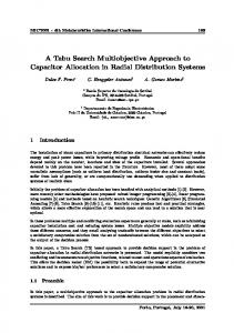
PS = {x ∈ Ω|x is Pareto optimal solution} and its image (i.e., PF = {F (x)|x ∈ PS}) is called Pareto Optimal Front. We are interested in maximizing the number of elements of the Pareto optimal set and maintaining a well-distributed set of solutions along the Pareto front. B. Decomposing Multi-objective Optimization Problems In the specialized literature, there are several approaches for transforming a MOP into multiple single-objective optimization subproblems [15]. These approaches use a weighted vector as their search direction. In this way and under certain assumptions (e.g. the minimum is unique, the weighting coefficients are positive, etc.), a Pareto optimal point is achieved by solving such subproblems. Among these methods, probably the two most widely used are the Tchebycheff and the Weighted Sum approaches. However, as it has been previously discussed in [3], [24], the approaches based on boundary intersection possess certain advantages over those based on either Tchebycheff or the Weighted Sum. In the following, we introduce a decomposition approach based on the boundary intersection, which is the approach adopted in this work. 1) Penalty Boundary Intersection Approach: The Penalty Boundary Intersection (PBI) approach2 was proposed by Zhang and Li [24], and uses a weighted vector w and a penalty value θ for minimizing both the distance to the utopian vector (d1 ) and the direction error to the weighted vector (d2 ) from the solution F (x) (see Fig. 1). Mathematically, the PBI problem can be stated as follows: Let w = (w1 , . . . , wkP )T be a weighted vector, i.e., wi ≥ 0 k for all i = 1, . . . , k and i=1 wi = 1. Then, the optimization problem is defined as: minimize: g(x|w, z ⋆ ) = d1 + θd2

(2)

such that: ||(F (x) − z ⋆ )T w|| ||w|| w d2 = (F (x) − z ⋆ ) − d1 ||w||

d1 = and

Attainable Objective Set

where x ∈ Rn , θ is the penalty value and z ⋆ = (z1⋆ , . . . , zk⋆ )T is the utopian vector, i.e., z ⋆ = min{fi (x)|x ∈ Ω} for each i = 1, . . . , k. 2 PBI is based on the well-known Normal Boundary Intersection (NBI) method [3]

Fig. 1.

Illustration of the Penalty Boundary Intersection (PBI) approach.

In this way, the PBI approach can generate a good approximation along the Pareto optimal front by defining a welldistributed set of weighted vectors. C. The Nonlinear Simplex Search Nelder and Mead’s method [16] also known as the Nonlinear Simplex Search (NSS), is an algorithm based on the simplex algorithm of Spendley et al. [20], which was introduced for minimizing nonlinear and multidimensional unconstrained functions. While Spendley et al.’s algorithm uses regular simplexes, Nelder and Mead’s method generalizes the procedure to change the shape and size of the simplex. Therefore, the convergence towards a minimum value at each iteration of the NSS method is conducted by three main movements in a geometric shape called simplex. The following definitions are of relevance here: Definition 4. A simplex or n-simplex ∆ is a convex hull of a set of n + 1 affinely independent points ∆i (i = 1, . . . , n + 1), in some Euclidean space of dimension n. Definition 5. A simplex is called nondegenerated, if and only if, the vectors in the simplex denote a linearly independent set. Otherwise, the simplex is called degenerated, and then, the simplex will be defined in a lower dimension than n. The full algorithm is defined stating three scalar parameters to control the movements performed in the simplex: reflection (α), expansion (γ) and contraction (β). At each iteration, the n + 1 vertices ∆i of the simplex represent solutions which are evaluated and sorted according to: f (∆1 ) ≤ f (∆2 ) ≤ · · · ≤ f (∆n+1 ). In this way, the movements performed in the simplex by the NSS method are defined as: 1) Reflection: xr = (1 + α)xc − α∆n+1 . 2) Expansion: xe = (1 + αγ)xc − αγ∆n+1 . 3) Contraction: a) Outside: xco = (1 + αβ)xc − αβ∆n+1 . b) Inside: xci = (1 − β)xc + β∆n+1 .

Pn where xc = n1 i=1 ∆i is the centroid of the n best points (all vertices except for ∆n+1 ), ∆1 and ∆n+1 are the best and the worst solutions identified within the simplex, respectively. Fig. 2 shows all the possible movements made by the NSS method. At each iteration, the initial simplex is modified by one of the above movements, according to the following rules: 1. If f (∆1 ) ≤ f (xr ) ≤ f (∆n ), then ∆n+1 = xr . 2. If f (xe ) < f (xr ) < f (∆1 ), then ∆n+1 = xe , otherwise ∆n+1 = xr . 3. If f (∆n ) ≤ f (xr ) < f (∆n+1 ) and f (xco ) ≤ f (xr ), then ∆n+1 = xco . 4. If f (xr ) ≥ f (∆n+1 ) and f (xci ) < f (∆n+1 ), then ∆n+1 = xci .

if it is not allocated in the same dimensionality as the simplex [11]. On the other hand, a degenerated simplex could be used to obtain local optimal solutions, at least, in the dimensionality defined by the simplex. In most real-world MOPs, the features of the Pareto optimal set are unknown. If the Pareto optimal set is contained in a lower dimension than the number of decision variables, then, the property that exists when using a degenerated simplex in the search could be exploited. Since the MOP is decomposed into several single-objective subproblems and assuming that each subproblem is solved throughout the search, then, the simplex could be constructed using such solutions. In this way, multiple approximate solutions to the Pareto optimal set are achieved while the search eventually converges to the region in which the Pareto set is contained. The convergence towards a better point given by the NSS method should be achieved at most in n+1 iterations (at least in convex functions with low dimensionality) [11]. Thus, a considerable number of function evaluations will be used to minimize each subproblem. Therefore, a good strategy for approximating solutions to the Pareto optimal set needs to be adopted. In this work, we take into account the above observations and design an effective nonlinear simplex search approach for solving MOPs. This strategy is described next. B. The Proposed Approach

Fig. 2. Illustration of the possible movements in the simplex performed by the NNS method. The constructed simplex corresponds to an optimization problem with two decision variables, where ∆1 and ∆3 are the best and the worst point, respectively.

III. T HE N ONLINEAR S IMPLEX S EARCH M ULTI - OBJECTIVE O PTIMIZATION

FOR

A. About the Nonlinear Simplex Search As indicated before, mathematical programming techniques are known to have several drawbacks with respect to evolutionary algorithms. The Nelder and Mead method has one more: the convergence towards an optimal value can fail when the simplexes elongate indefinitely and their shape goes to infinity in the space of simplex shapes (as, for example, in McKinnon’s functions [14]). For this family of functions and others having similar features, a more appropriate strategy needs to be adopted (e.g., adjusting the control parameters, constructing in a different way the simplex, improving heuristically the movements of the NSS method, etc.). In recent years, several attempts to improve the NNS method have been reported in the literature (see for example [22], [17]). Also, different strategies for the construction of the simplex were explored in [1], [23]. The construction of the simplex plays an important role in the performance of the NSS method. To employ a degenerated simplex (i.e., to use a simplex defined in a lower dimension than the number of decision variables) in the minimization process, is not a good idea. That is because the search is restricted to find an optimal solution in a lower dimension, which avoids achieving this optimal solution

Our proposed Nonlinear Simplex Search for Multiobjective Optimization (NSS-MO), decomposes a MOP into several single-objective scalarization subproblems. Therefore, a well-distributed set of weighted vectors W = {w1 , . . . , wN } has to be previously defined. Here, we use the same method as in [24], however, other methods can be used, see for example [2]. At the beginning, a set of N solutions S = {x1 , . . . , xN } is randomly initialized. Each solution xi ∈ S minimizes the ith subproblem defined by the ith weighted vector wi ∈ W . In this way, different subproblems are solved by the NSS-MO algorithm and the leading set (i.e. the set S) will approximate solutions towards the Pareto optimal set lengthwise of the search process. The search is directed towards different non-overlapped regions (or partitions) Ci ’s from the set of weighted vectors W , such that, each Ci defines a neighborhood. That is, let C = {C1 , . . . , Cm } be a set of partitions from W , then, the claim is the following: m \

i=1

Ci = ∅ and

m [

Ci = W

(3)

i=1

and all the weighted vectors wc ∈ Ci are contiguous among themselves. Thus, the NSS method is focused on minimizing a subproblem defined by a weighted vector ws which is randomly chosen from Ci . The n-simplex (∆) used in the search, is defined as: ∆ = {xs , x1 , . . . , xn } (4) such that: xs ∈ S is a minimum of g(xs |ws , z ⋆ ) for any ws ∈ W . xj ∈ S represents the n solutions that minimize the

Algorithm 1 update(W, S, I) 1: T = S ∪ I; 2: R = ∅; 3: for all wi ∈ W do 4: R = R ∪ {x⋆ | min g(x⋆ |wi , z ⋆ )}; ⋆ 5: 6: 7:

⋆

C1 C2 C3 C4 C5 C6

1

1

x ∈T

T = T \ {x }; end for return R;

C7 C8 C9 C10 C11

0 Search Direction (ws )

subproblems defined by the nearest n weighted vectors of ws , where j = 1, . . . , n and n represents the number of decision variables of the MOP. After a movement made by the NSS method, it is common that the new solution obtained, xn , leaves the search space. In order to deal with this problem, (as in [23]) we bias deterministically the boundaries. Therefore, the ith bound of the new solution xn is re-established as follows: ( xilb , if xin < xilb i xn = (5) xiub , if xin > xiub where xilb and xiub are, respectively, the lower and upper bounds in the ith component of the search space. The search could be relaxed at each iteration by changing the direction vector for any other direction w ˆs ∈ Ci . With this, we get an agile search into the partition Ci and we avoid collapsing the simplex search in the same direction ws . |W | partitions of the set W , Here, we define m = n+1 guaranteeing at least n + 1 iterations of the NSS method for each partition, which can be constructed using a naive modification of the well-known k-means algorithm [13]. Then, we say that one iteration of our NSS-MO has been carried out, when the NSS method iterates n + 1 times in each defined partition Ci . Therefore, at each iteration the proposed algorithm performs |W | function evaluations. All of the new solutions found in the search process are stored in a pool called intensification set (I). Then, at the end of each iteration, the leading set S is updated using both the intensification set I and the weighted set W , such as it is shown in Algorithm 1. With this, the NSS method minimizes each subproblem, generating new search trajectories among the solutions of the simplex, while the updating mechanism replaces the misguided paths by selecting the best solutions according to the PBI approach, simulating the Path Relinking method [7]. In Fig. 3, we show a possible partition of the weighted set W for a MOP with three objective functions and five decision variables, i.e. defining an n-simplex with six vertices. Summarizing, the NSS-MO algorithm can be stated as follows: Step 1) Initialization Step 1.1) t = 0 // the number of iterations Step 1.2) Generate a well-distributed set of weighted vectors W = {w1 , . . . , wN } of N .

1

The n-simplex

Fig. 3. Illustration of a well-distributed set of weighted vectors for a MOP with three objectives, five decision variables and 66 weighted vectors, i.e. |W | m = n+1 = 11 partitions. The n-simplex is constructed by six solutions contained in four different partitions (C5 , C8 , C9 and C10 ). The search is focused on the direction defined by the weighted vector ws .

Step 1.3) Generate the leading set S t = {x1 . . . , xN } of N random solutions. |w| Step 1.4) Generate partitions: Generate m = n+1 partitions C = {C1 , . . . , Cm } from W (where n is the number of decision variables), such that: the eq.( 3) is satisfied. Step 2) The iteration // Generate the intensification set I I=∅ For i = 1, . . . , m, do // for each partition Ci ∈ C 2.1) Randomly choose ws ∈ Ci 2.2) Apply Nelder and Mead’s method: 2.2.1) Build the n-simplex: Construct the nsimplex from S t , such that: eq.( 4) is satisfied. 2.2.2) Apply the NSS method: Execute the NSS method during n+1 iterations. At each iteration: · Repair the bounds according to eq.( 5). · Relax the search changing the direction search ws for any other w ˆ s ∈ Ci . · Each new solution found by the NSS method is stored in the intensification set I.

Step 3) Update the leading set: Update the leading set S using Algorithm 1. That is: S t+1 = update(W, S t , I) Step 4) Stopping Criteria: If t < Nit (Nit is the maximum number of iterations) then t = t + 1 and go to Step 2. Otherwise, stop NSS-MO and output: S t+1 . IV. T EST P ROBLEMS In order to assess the performance of the proposed approach, we compare its results with respect to those obtained by a state-of-the-art MOEA called MOEA/D [24]. We adopted three benchmark problems (LIS, FONSECA and DTLZ5) and an airfoil design problem as a case study. Next, we present the description of such problems. A. Standard Test Problems The following standard test problems were used to assess the performance of our proposed approach.

TABLE I PARAMETER RANGES FOR MODIFIED PARSEC AIRFOIL LIS [12]:

f1 (x)

=

f2 (x)

=

q 8 x21 + x22 p 4 (x1 − 0.5)2 + (x2 − 0.5)2

where xi ∈ [−5, 10]. This MOP has a concave and connected Pareto front. FONSECA [6]:

f1 (x) f2 (x)

= =

P 1 − exp(− n (xi − Pi=1 1 − exp(− n i=1 (xi +

√1 )2 ) n) √1 )2 ) n)

where n = 3 and xi ∈ [−4, 4]. This MOP has a concave and connected Pareto front. DTLZ5 [4]:

f1 (x) f2 (x) f3 (x) θ1 θ2 g(x) h(x)

= = = = = = =

cos(θ1 ) cos(θ2 )h(x) cos(θ1 ) sin(θ2 )h(x) sin(θ1 )h(x) π 2 x1 π (1 + 2g(x)x2 ) 4(1+g(x)) P n 2 i=k (xi − 0.5) 1 + g(x)

where k = 3, n = 12 and xi ∈ [0, 1]. This MOP has a degenerated Pareto front formed by a curve of welldistributed solutions. B. Airfoil Shape Optimization: A case study Our case study consists of the multi-objective optimization of an airfoil shape problem adapted from [21] (called here MOPRW). This problem corresponds to the airfoil shape optimization of a standard-class glider, aiming to obtain an optimum performance for a sailplane. In this study the tradeoff among two aerodynamic objectives is evaluated using our proposed approach, and its results are compared with respect to those obtained by MOEA/D. 1) Problem Statement: Two conflicting objective functions are defined in terms of a sailplane average weight and operating conditions [21]. They are defined as: i) minimize: CD /CL s.t. CL = 0.63, Re = 2.04 · 106 , M = 0.12 3/2 ii) minimize: CD /CL s.t. CL = 1.05, Re = 1.29 · 106 , M = 0.08 3/2 where CD /CL and CD /CL correspond to the inverse of the glider’s gliding ratio and sink rate, respectively. Both are important performance measures for this aerodynamic optimization problem. CD and CL are the drag and lift coefficients. The aim is to maximize the gliding ratio (CL /CD ) for objective (i), while minimizing the sink rate in objective (ii). Each of these objectives is evaluated at different prescribed flight conditions, given in terms of Mach and Reynolds numbers. The aim of solving this MOP is to find a better airfoil shape, which improves a reference design. 2) Geometry Parametrization: In the present case study, the PARSEC airfoil representation [19] was adopted. Fig. 4 illustrates the 11 basic parameters used for this representation: rle leading edge radius, Xup /Xlo location of maximum thickness for upper/lower surfaces, Zup /Zlo maximum thickness for upper/lower surfaces, Zxxup /Zxxlo curvature for upper/lower surfaces, at maximum thickness locations, Zte trailing edge coordinate, ∆Zte trailing edge thickness, αte trailing edge direction, and βte trailing edge wedge angle.

REPRESENTATION

Design Variable rleup rlelo αte βte Zte ∆Zte Xup Zup Zxxup Xlo Zlo Zxxlo

Lower Bound 0.0085 0.0020 7.0000 10.0000 -0.0060 0.0025 0.4100 0.1100 -0.9000 0.2000 -0.0230 0.0500

Upper Bound 0.0126 0.0040 10.0000 14.0000 -0.0030 0.0050 0.4600 0.1300 -0.7000 0.2600 -0.0150 0.2000

For the present case study, the modified PARSEC geometry representation adopted allows us to define independently the leading edge radius, both for upper and lower surfaces. Thus, a total of 12 variables are used. Their allowable ranges are defined in Table I. The PARSEC airfoil geometry representation uses a linear combination of shape functions for defining the upper and lower surfaces. These linear combinations are given by:

Zupper =

6 X

an x

n−1 2

,

Zlower =

n=1

6 X

bn x

n−1 2

(6)

n=1

In the above equations, the coefficients an , and bn are determined as functions of the 12 described geometric parameters, by solving two systems of linear equations, one for each surface. It is important to note that the geometric parameters rleup /rlelo , Xup /Xlo , Zup /Zlo , Zxxup /Zxxlo , Zte , ∆Zte , αte , and βte are the actual design variables in the optimization process, and that the coefficients an , bn serve as intermediate variables for interpolating the airfoil’s coordinates, which are used by the CFD solver (we used the Xfoil CFD code [5]) for its discretization process. V. C OMPARISON

OF

R ESULTS

A. Performance Measures 1) Hypervolume: The Hypervolume (Hv) metric was proposed by Zitzler [25]. This performance measure is Pareto compliant [26] and quantifies the approximation of nondominated solutions to the Pareto optimal front. The hypervolume corresponds to the non-overlapped volume of all the hypercubes formed by a reference point r (given by

Fig. 4.

PARSEC airfoil parametrization.

the user) and each solution p in the Pareto set approximation (PF k ). It is mathematically defined as:   [ Hv = Λ  {x|p ≺ x ≺ r} (7) p∈PF k

where Λ denotes the Lebesgue measure and r ∈ Rk denotes a reference vector being dominated by all valid candidate solutions in P Fk . 2) Spacing: The Spacing (Sp) metric proposed by Schott [18], quantifies the spread of solutions in the obtained approximation of the Pareto front. This performance measure can be calculated as: v u |P | u 1 X t (8) (d − di )2 Sp = |P | i=1 where di and d are defined as: di = min

i,i6=j

M X

k=1

|fki − fkj |, and d =

TABLE II PARAMETERS FOR NSS-MO AND MOEA/D Parameter Nsol Nit Tn Pc Pm α β γ θ

R ESULTS OF THE Hv

MOP LIS FONSECA DTLZ5

P|P |

i=1

di

MOPRW

NSS-MO 100/300 40 – – – 1 2 0.5 5

MOEA/D 100/300 40 30 1 1/n – – – 5

TABLE III NSS-MO AND MOEA/D

METRIC FOR

NSS-MO average (σ) 0.309713 (0.007686) 0.542006 (0.001476) 0.429676 (0.000917) 2.055961e-07 (3.045320e-08)

MOEA/D average (σ) 0.262384 (0.008786) 0.374342 (0.007427) 0.425734 (0.001480) 2.045719e-07 (2.511415e-08)

|P |

A value of zero for this performance measure indicates that all the solutions are uniformly spread (i.e., the best possible performance). B. Experimental Setup As indicated before, we compared our proposed approach with respect to MOEA/D [24] (which uses the PBI approach). For each MOP, 30 independent runs were performed with each approach. The parameters for both algorithms are summarized in Table II, where Nsol represents the number of initial solutions (100 for bi-objective problems and 300 for three-objective problems). Nit represents the number of iterations (which was set to 40). Therefore, we performed 4, 000 (for the bi-objective problems) and 12, 000 (for the three-objective problems) function evaluations. For NSSMO, α, β and γ represent the control parameters for the reflection, expansion and contraction movements of the NSS method. For MOEA/D, the parameters Tn , ηc , ηm , Pc and Pm represent the neighborhood size, crossover index, mutation index, crossover rate and mutation rate, respectively. Finally, the parameter θ, represents the penalty value used in the PBI approach for both the NSS-MO and MOEA/D. For each MOP, the algorithms were evaluated using the two performance measures previously defined. (Hypervolume and Spacing). Regarding the hypervolume, the reference vectors adopted were: r = (1, 1)T for the LIS problem, and r = (1.1, . . . , 1.1)T for the FONSECA and DTLZ5 problems, while for the airfoil design problem the reference vector r = (0.007610, 0.005236)T was employed. The results obtained are summarized in Tables III and IV. Each table displays both the average and the standard deviation (σ) of each performance measure for each MOP. For an easier interpretation, the best results are presented in boldface for each performance measure and test problem adopted.

TABLE IV R ESULTS OF THE Sp METRIC FOR NSS-MO AND MOEA/D

MOP LIS FONSECA DTLZ5 MOPRW

NSS-MO average (σ) 0.005861 (0.000812) 0.004454 (0.000218) 0.007064 (0.001211) 1.554402e-05 (7.141540e-06)

MOEA-D average (σ) 0.010273 (0.003768) 0.003346 (0.000498) 0.034209 (0.031652) 2.397431e-06 (2.790701e-06)

C. Results and Discussion In this section, we present the results obtained by the proposed algorithm for each adopted test problem including the airfoil design problem. As indicated before, the results obtained by our proposed approach (NSS-MO) are compared against those produced by MOEA/D. Table III shows the results obtained for the hypervolume (Hv) performance measure. From this table, it can be seen that the results obtained by our proposed approach outperformed MOEA/D in all the adopted MOPs. This indicates that our proposed algorithm produced a better approximation to the Pareto optimal front. Regarding the spacing (Sp) performance measure, Table IV shows that MOEA/D obtained better results than those produced by our proposed NSS-MO in the FONSECA and MOPRW problems, while NSS-MO was better in the LIS and DTLZ5 test problems. However, in our case, convergence was considered to be a more important criterion than uniform distribution, and regarding convergence, our proposed approach obtained better results in all cases. Fig. 5 graphically shows that NSS-MO obtained both a better distribution of solutions and a better approximation

PARETO FRONT NSS−MO MOEA/D

PARETO FRONT NSS−MO MOEA/D

PARETO FRONT NSS−MO MOEA/D

f2

f2

f3

f1 f2 f1

f1

A) NSS-MO and MOEA/D in LIS problem

B) NSS-MO and MOEA/D in FONSECA problem

C) NSS-MO and MOEA/D in DTLZ5 problem

0.6

0.35

0.5 NSS−MO MOEA/D

NSS−MO MOEA/D

NSS−MO MOEA/D

0.55

0.45

0.3 0.5 0.25

0.4

0.45

0.2

0.15

Hypervolume

Hypervolume

Hypervolume

0.35 0.4 0.35 0.3

0.3

0.25

0.2 0.25

0.1

0.15

0.2 0.05

0.1

0.15 0.1

0 5

10

15

20

25 Generation

30

35

40

45

0.05 5

50

D) Hypervolume convergence for LIS problem

10

15

20

25 Generation

30

35

40

45

50

E) Hypervolume convergence for FONSECA problem

5

10

15

20

25 Generation

30

35

40

45

50

F) Hypervolume convergence for DTLZ5 problem

Fig. 5. Comparison of results for NSS-MO and MOE/D in the benchmark problems. Figures A to C show the achieved Pareto front, while Figures D to F show the convergence plot of the hypervolume for the LIS, FONSECA and DTLZ5 problems, respectively. 0.0053

0.0051

0.0051

NSS−MO MOEA/D

NSS−MO MOEA/D

0.00525

NSS−MO MOEA/D

0.00508

0.00508

0.00506

0.00506

0.00504

0.00504

0.0052

f_2

f_2

f_2

0.00515 0.00502

0.00502

0.0051 0.005

0.005

0.00498

0.00498

0.00496

0.00496

0.00505

0.005

0.00495 0.0066

0.0067

0.0068

0.0069

0.007

0.0071

0.0072

0.00494 0.0066

0.0073

0.00665

0.0067

0.00675

f_1

0.0068

0.00685

0.0069

0.00695

0.00494 0.0066

0.007

A) NSS-MO and MOEA/D in MOPRW after 10 generations

0.0067

0.00675

0.0068

0.00685

0.0069

0.00695

0.007

0.00705

f_1

B) NSS-MO and MOEA/D in MOPRW after 20 generations

0.00508

C) NSS-MO and MOEA/D in MOPRW after 30 generations

2.4e−07 NSS−MO MOEA/D

NSS−MO MOEA/D

2.2e−07

2.4e−07

2e−07 0.00504

1.8e−07

2.1e−07

1.6e−07

1.8e−07

1.4e−07

Hypervolume

Hypervolume

0.00502

0.005

NSS−MO MOEA/D

2.7e−07

0.00506

f_2

0.00665

f_1

1.2e−07 1e−07

1.5e−07 1.2e−07

0.00498 8e−08 0.00496

9e−08

6e−08 6e−08 4e−08

0.00494

3e−08

2e−08 0.00492 0.0066

0 0.00665

0.0067

0.00675

0.0068 0.00685 f_1

0.0069

0.00695

0.007

D) NSS-MO and MOEA/D in MOPRW after 40 generations

0.00705

0 5

10

15

20

25 30 Generation

35

40

45

50

E) Hypervolume convergence for MOPRW problem after 50 generations

10

20

30

40

50 Generation

60

70

80

90

100

F) Hypervolume convergence for MOPRW problem after 100 generations

Fig. 6. Comparison of results for NSS-MO and MOE/D in the airfoil design problem. Figures A to D compare the achieved Pareto front for 10, 20, 30 and 40 generations, while figures E and F show the convergence plot of the hypervolume at 50 and 100 generations, respectively.

to the Pareto optimal front in the LIS and FONSECA test problems. The differences in the distribution of solutions for DTLZ5 do not seem significant when comparing the two approaches, although MOEA/D was better in this case. It is worth noting that both approaches converged to the true Pareto front, but their approximations are shown at different positions in Fig. 5 to make them more readable. That is the reason why the axes of these plots do not have any numerical values. Fig. 6 shows the approximation of the Pareto front generated by both NSS-MO and MOEA/D after 10, 20, 30 and

40 iterations. In this case, NSS-MO obtained, on average, better hypervolume values than MOEA/D (see Table III), although the difference is not significant. In fact, Fig. 6 shows a particular instance in which MOEA/D obtained a better hypervolume value than our approach after 100 iterations. The approximations to the Pareto front presented in Figs. 5 and 6, correspond to the set of nondominated solutions found by each algorithm in the run with the value nearest to the mean value of the Hv metric for each multi-objective optimization problem adopted.

VI. C ONCLUSIONS

AND

F UTURE W ORK

We have proposed a multi-objective algorithm based on mathematical programming techniques. The proposed approach was, in principle, designed for dealing with unconstrained, and unimodal problems having low and moderate dimensionality. Our results indicate that our proposed NSS-MO algorithm outperforms MOEA/D regarding convergence in all the test problems adopted, including one from aeronautical engineering. The number of objective function evaluations in these test problems was low (4,000 for the bi-objective problems and 12,000 for the three-objective problems), which can make it a good choice for dealing with expensive objective functions. Our proposed approach has, however, some disadvantages. For example, when dealing with highly accidented search spaces, the movements of the NSS method may not be able to reach a better point during the search. Should that be the case, the step sizes (i.e., the control parameters α, β and γ) must be fine-tuned until finding a suitable search region. In spite of the effectiveness of our proposed approach in MOPs with moderate dimensionality, our main goal is to hybridize it with a MOEA so that its use can be extended to problems of higher dimensionality and with highly accidented search spaces. The idea would be to use a MOEA for locating promising regions of the search space, and then apply NSS-MO for exploiting those regions in an efficient way. We believe that this sort of multi-objective memetic algorithm could be a powerful engine for solving complex and computationally expensive MOPs. ACKNOWLEDGEMENTS The first author acknowledges support from CONACyT through a scholarship to pursue graduate studies at the Computer Science Department of CINVESTAV-IPN. The second author acknowledges support from IPN and CONACyT to pursue graduate studies at the Computer Science Department of CINVESTAV-IPN The third author gratefully acknowledges support from CONACyT project no. 103570.

R EFERENCES [1] R. Chelouah and P. Siarry. Genetic and Nelder-Mead algorithms hybridized for a more accurate global optimization of continuous multiminima functions. European Journal of Operational Research, 148(2):335–348, July 2003. [2] I. Das. Nonlinear Muicriteria Optimization and Robust Optimality. PhD thesis, Rice University, Houston, Texas, 1997. [3] I. Das and J. E. Dennis. Normal-boundary intersection: a new method for generating Pareto optimal points in multicriteria optimization problems. SIAM Journal on Optimization, 8(3):631–657, 1998. [4] K. Deb, L. Thiele, M. Laumanns, and E. Zitzler. Scalable Test Problems for Evolutionary Multiobjective Optimization. In A. Abraham, L. Jain, and R. Goldberg, editors, Evolutionary Multiobjective Optimization. Theoretical Advances and Applications, pages 105–145. Springer, USA, 2005. [5] M. Drela. XFOIL: An Analysis and Design System for Low Reynolds Number Aerodynamics. In Conference on Low Reynolds Number Aerodynamics, University Of Notre Dame, IN, June 1989. [6] C. M. Fonseca and P. J. Fleming. Multiobjective Genetic Algorithms Made Easy: Selection, Sharing, and Mating Restriction. In Proceedings of the First International Conference on Genetic Algorithms in Engineering Systems: Innovations and Applications, pages 42–52, Sheffield, UK, September 1995. IEE.

[7] F. Glover. Tabu search and adaptive memory programing – Advances, applications and challenges. In Interfaces in Computer Science and Operations Research, pages 1–75. Kluwer Academic Publishers, 1996. [8] C. K. Goh, Y. S. Ong, K. C. Tan, and E. J. Teoh. An Investigation on Evolutionary Gradient Search for Multi-Objective Optimization. In 2008 Congress on Evolutionary Computation (CEC’2008), pages 3742–3747, Hong Kong, June 2008. IEEE Service Center. [9] A. G. Hern´andez-D´ıaz, C. A. Coello Coello, F. P´erez, R. Caballero, J. Molina, and L. V. Santana-Quintero. Seeding the Initial Population of a Multi-Objective Evolutionary Algorithm using GradientBased Information. In 2008 Congress on Evolutionary Computation (CEC’2008), pages 1617–1624, Hong Kong, June 2008. IEEE Service Center. [10] P. Koduru, S. Das, and S. M. Welch. Multi-Objective Hybrid PSO Using ǫ-Fuzzy Dominance. In D. Thierens, editor, 2007 Genetic and Evolutionary Computation Conference (GECCO’2007), volume 1, pages 853–860, London, UK, July 2007. ACM Press. [11] J. C. Lagarias, J. A. Reeds, M. H. Wright, and P. E. Wright. Convergence properties of the Nelder–Mead simplex method in low dimensions. SIAM Journal of Optimization, 9:112–147, 1998. [12] J. Lis and A. E. Eiben. A Multi-Sexual Genetic Algorithm for Multiobjective Optimization. In T. Fukuda and T. Furuhashi, editors, Proceedings of the 1996 International Conference on Evolutionary Computation, pages 59–64, Nagoya, Japan, 1996. IEEE. [13] J. B. MacQueen. Some Methods for Classification and Analysis of Multivariate Observations. In Proceedings of the fifth Berkeley Symposium on Mathematical Statistics and Probability, volume 1, pages 281–297. University of California Press, 1967. [14] K. I. M. McKinnon. Convergence of the Nelder–Mead Simplex Method to a Nonstationary Point. SIAM Journal on Optimization, 9(1):148–158, 1998. [15] K. Miettinen. Nonlinear Multiobjective Optimization. Kluwer Academic Publishers, Boston, Massachuisetts, 1999. [16] J. A. Nelder and R. Mead. A Simplex Method for Function Minimization. The Computer Journal, 7:308–313, 1965. [17] M. K. Rahman. An intelligent moving object optimization algorithm for design problems with mixed variables, mixed constraints and multiple objectives. Structural and Multidisciplinary Optimization, 32(1):40–58, July 2006. [18] J. R. Schott. Fault Tolerant Design Using Single and Multicriteria Genetic Algorithm Optimization. Master’s thesis, Department of Aeronautics and Astronautics, Massachusetts Institute of Technology, Cambridge, Massachusetts, May 1995. [19] H. Sobieczky. Parametric Airfoils and Wings. In K. Fuji and G. S. Dulikravich, editors, Notes on Numerical Fluid Mechanics, Vol.. 68, pages 71–88, Wiesbaden, 1998. Vieweg Verlag. [20] W. Spendley, G. R. Hext, and F. R. Himsworth. Sequential Application of Simplex Designs in Optimization and Evolutionary Operation. Technometrics, 4(4):441–461, November 1962. [21] A. Sz¨oll¨os, M. Sm´ıd, and J. H´ajek. Aerodynamic optimization via multi-objective micro-genetic algorithm with range adaptation, knowledge-based reinitialization, crowding and epsilon-dominance. Advances in Engineering Software, 40(6):419–430, 2009. [22] M. B. Trabia and X. B. Lu. A Fuzzy Adaptive Simplex Search Optimization Algorithm. Journal of Mechanical Design, 123:216–225, 2001. [23] S. Zapotecas Mart´ınez and C. A. Coello Coello. A Proposal to Hybridize Multi-Objective Evolutionary Algorithms with Non-Gradient Mathematical Programming Techniques. In G. Rudolph, T. Jansen, S. Lucas, C. Poloni, and N. Beume, editors, Parallel Problem Solving from Nature–PPSN X, volume 5199, pages 837–846. Springer. Lecture Notes in Computer Science, Dortmund, Germany, September 2008. [24] Q. Zhang and H. Li. MOEA/D: A Multiobjective Evolutionary Algorithm Based on Decomposition. IEEE Transactions on Evolutionary Computation, 11(6):712–731, December 2007. [25] E. Zitzler and L. Thiele. Multiobjective Optimization Using Evolutionary Algorithms—A Comparative Study. In A. E. Eiben, editor, Parallel Problem Solving from Nature V, pages 292–301, Amsterdam, September 1998. Springer-Verlag. [26] E. Zitzler, L. Thiele, M. Laumanns, C. M. Fonseca, and V. G. da Fonseca. Performance Assessment of Multiobjective Optimizers: An Analysis and Review. IEEE Transactions on Evolutionary Computation, 7(2):117–132, April 2003.