A NONLINEAR TEST MODEL FOR FILTERING SLOW ... - Project Euclid

c 2008 International Press °

COMMUN. MATH. SCI. Vol. 6, No. 3, pp. 611–649

A NONLINEAR TEST MODEL FOR FILTERING SLOW-FAST SYSTEMS∗ BORIS GERSHGORIN† AND ANDREW MAJDA‡ Abstract. A nonlinear test model for filtering turbulent signals from partial observations of nonlinear slow-fast systems with multiple time scales is developed here. This model is a nonlinear stochastic real triad model with one slow mode, two fast modes, and catalytic nonlinear interaction of the fast modes depending on the slow mode. Despite the nonlinear and non-Gaussian features of the model, exact solution formulas are developed here for the mean and covariance. These formulas are utilized to develop a suite of statistically exact extended Kalman filters for the slow-fast system. Important practical issues such as filter performance with partial observations, which mix the slow and fast modes, model errors through linear filters for the fast modes, and the role of observation frequency and observational noise strength are assessed in unambiguous fashion in the test model by utilizing these exact nonlinear statistics. Key words. Nonlinear model, slow-fast system, extended Kalman filter AMS subject classifications. 60H10, 60G35

1. Introduction Many contemporary problems in science and engineering involve large dimensional turbulent nonlinear systems with multiple time scales, i.e., slow-fast systems. The increasing need for real time predictions, for example, in extended range forecasting of weather and climate, drives the development of improved strategies for data assimilation or filtering [7, 13, 6, 10, 2, 3, 28, 4, 14]. Such filtering algorithms are based on generalizations of the classical Kalman filter [1, 5]. Filtering combines partially observed features of the chaotic turbulent multiscale signal together with a dynamic model to obtain a statistical estimate for the state of the system. The dynamic models for the coupled atmosphere-ocean system are prototype examples of slow-fast systems where the slow modes are advective vortical modes and the fast modes are inertia-gravity waves [29, 9, 21]. Depending on the spatio-temporal scale, one might need only a statistical estimate of the slow modes, as on synoptic scales in the atmosphere [7] or both slow and fast modes such as for squall lines on mesoscales due to the impact of moist convection [17]. In either situation, the noisy partial observations of quantities such as temperature, pressure, and velocity necessarily mix both the slow and fast modes [7, 6, 21]. Furthermore, the dynamical models often suffer from significant model errors due to lack of resolution or inadequate parametrization of physical processes such as clouds, moisture, boundary layers, and topography. The goal of the present paper is to develop a simple three dimensional nonlinear test model with exactly solvable statistics for slow-fast systems in order to provide unambiguous guidelines for the difficult issues for filtering slow-fast systems from partial observations, as mentioned in the first paragraph. Here, we also study filter performance and model errors in this idealized low-dimensional setting for slow-fast filtering; this study parallels earlier works [11, 26] using low dimensional nonlinear models of Lorenz [19, 20] or their variants [27] without exact statistical solutions to ∗ Received:

March 17, 2008; accepted (in revised version): June 4, 2008. Communicated by Shi

Jin. † Dept. of Mathematics and Center matical Sciences, New York University ‡ Dept. of Mathematics and Center matical Sciences, New York University

for Atmosphere Ocean Science, Courant Institute of Mathe([email protected]). for Atmosphere Ocean Science, Courant Institute of Mathe([email protected]). 611

612

A NONLINEAR TEST MODEL FOR FILTERING SLOW-FAST SYSTEMS

study nonlinear filter performance. However, here we have the additional advantage that with the exactly solvable statistics for the mean and covariance in the nonlinear non-Gaussian slow-fast test model, we can utilize a perfect extended Kalman filter algorithm [1] without additional Monte Carlo errors due to finite ensemble size. 1.1. The nonlinear test model for slow-fast systems. The nonlinear test model, which we propose here as a prototype for filtering slow-fast systems, is three dimensional with stochastic equations for the real slow mode, u1 , and the complex fast mode, u2 , given by the stochastic triad model, du1 = (−γ1 u1 + f1 (t))dt + σ1 dW1 , ³ ´ du2 = (−γ2 + iω0 /ε + ia0 u1 )u2 + f2 (t) dt + σ2 dW2 .

(1.1) (1.2)

In equations (1.1) and (1.2), ε is a small parameter that measures the deterministic time scale ratio between the evolution of the fast and slow waves; the damping coefficients, γ1 and γ2 , and white noise forcings represent the turbulent interaction and energy transfer through nonlinear interaction with other unresolved modes in the triad model [29, 24, 25]; the parameter a0 measures the nonlinearity in the system, in which energy is always conserved; the terms f1 (t), f2 (t) represent deterministic forcing of the slow and fast modes, respectively. The nonlinear test model in equations (1.1) and (1.2) is motivated directly by both the mathematical theory of slow-fast geophysical flows [9, 21] and high resolution turbulent simulations in slow-fast geophysical regimes [30, 31, 32]; all this work suggests that the slow vortical mode dynamics, u1 here, and the nonlinear catalytic interactions of the slow modes with the fast modes, u2 here, are the most important central nonlinear features of slow-fast interaction for geophysical systems. The model in equations (1.1) and (1.2) is the simplest one which retains these nonlinear features. In the present paper, we set f2 (t) ≡ 0 for simplicity, thus we ignore explicit forcing for the fast waves. In section 2, we develop exactly solvable solution formulas for the nonlinear, non-Gaussian statistical solutions for equations (1.1) and (1.2) by generalizing and extending the exact solutions for the Kubo oscillator from statistical physics [18, 23] to non-stationary and cross-correlated dynamics. In section 3, we set up idealized extended Kalman filter algorithms, which utilize the exact solution formulas developed in section 2. In section 4, we study filter performance and model error for the test model in a framework motivated by all the practical issues for filtering slow-fast systems mentioned in the first paragraph. The paper ends with a brief concluding discussion. 2. Exact solutions and exactly solvable statistics in the nonlinear test model 2.1. Model. As presented in the introduction, consider a system of one slow wave represented by a real-valued function u1 and two fast waves represented by a complex-valued function u2 . We model this system via a system of coupled stochastic differential equations of the form du1 = (−γ1 u1 + f1 (t))dt + σ1 dW1 , du2 = (−γ2 + iω0 /ε + ia0 u1 )u2 dt + σ2 dW2 ,

(2.1) (2.2)

where γ1 and γ2 are the damping coefficients of the slow and fast waves, respectively, f1 (t) is forcing of the slow wave, σ1 and σ2 represent the strength of the noise of

613

BORIS GERSHGORIN AND ANDREW MAJDA

the slow and fast waves, respectively, ε is a small parameter that characterizes the time scale difference between the slow and the fast modes, ω0 is typical frequency of the fast wave in the units of ε, and a0 is a nonlinearity parameter. We choose the oscillatory forcing f1 (t) = Asin(ωt). The system (1.1)–(1.2) is to be solved with the initial conditions u1 (t0 ) = u10 , u2 (t0 ) = u20 , where u10 and u20 are correlated Gaussian random variables with known parameters: hu10 i, hu20 i, Var(u10 ), Var(u20 ), Cov(u20 ,u∗20 ) and Cov(u20 ,u10 ). As usual, h·i is expectation, Var(·) is variance, and Cov(·,·) is covariance. 2.2. Path-wise solution of the model. It is not difficult to develop pathwise solutions of the model equations. Such path-wise solutions provide the signals, which we attempt to filter. First we solve equation (1.1) since it is independent of the fast wave u2 . The slow wave u1 is easily found using an integrating factor −γ1 (t−t0 )

u1 (t) = u10 e

+ F1 (t) + σ1

Z

t

eγ1 (s−t) dW1 (s),

(2.3)

t0

where F1 (t) =

Z

t

f1 (s)e−γ1 (t−s) ds

t0

=

A

γ12 + ω 2

³

´ ¡ ¢ e−γ1 (t−t0 ) ω cos(ωt0 ) − γ1 sin(ωt0 ) − ω cos(ωt) + γ1 sin(ωt) .

Note that u1 (t) is a Gaussian random process, and thus is fully defined by its mean and variance, which will be computed below. Now, to solve equation (1.2) we treat u1 as a known function. Using the integrating factor for the equation with time-dependent frequency, we obtain u2 u2 (t) = e−γ2 (t−t0 ) ψ(t0 ,t)u20 + σ2

Z

t

e−γ2 (t−s) ψ(s,t)dW2 (s),

(2.4)

t0

where we defined new functions ψ(s,t) = eiJ(s,t) , Z t Z t³ ´ u1 (s′ )ds′ ω0 /ε + a0 u1 (s′ ) ds′ = (t − s)ω0 /ε + a0 J(s,t) = s

= JD (s,t) + JW (s,t) + b(s,t)u10 ,

s

(2.5)

where the deterministic part of J(s,t) is Ã ´ ³ ´ Aa0 γ1 ³ JD (s,t) = (t − s)ω0 /ε + 2 cos(ωs) − cos(ωt) + sin(ωs) − sin(ωt) γ1 + ω 2 ω ¶! ´µ ω ³ + e−γ1 (s−t0 ) − e−γ1 (t−t0 ) cos(ωt0 ) − sin(ωt0 ) , γ1

614


the noisy part of J(s,t) is JW (s,t) = σ1 a0

Z

t

ds

s

′

Z

s′

eγ1 (s

′′

−s′ )

dW1 (s′′ ),

t0

and the prefactor of u10 is b(s,t) =

´ a0 ³ −γ1 (s−t0 ) e − e−γ1 (t−t0 ) . γ1

Note that J(s,t) linearly depends on u1 and, therefore, J(s,t) is also a sum of independent Gaussian random fields. We also introduce the following notation for later use ψD (s,t) = eiJD (s,t) , ψW (s,t) = eiJW (s,t) . On the other hand, u2 is not a Gaussian random variable in the case a0 6= 0, because the solution formula involves exponentials of Gaussian random variables. Below, we will confirm nongaussianity of u2 numerically. Nevertheless, we will be able to compute the statistics of u2 analytically due to the special structure of the solution. 2.3. Invariant measure and choice of parameters. Here, we obtain the invariant measure of (1.1)–(1.2) without forcing. We separate (1.1)–(1.2) into two parts: the deterministic part, du1 = 0,

(2.6)

du2 = i(ω0 /ε + a0 u1 )u2 dt,

(2.7)

and the randomly fluctuating and damped part, du1 = −γ1 u1 dt + σ1 dW1 ,

du2 = −γ2 u2 dt + σ2 dW2 .

(2.8) (2.9)

Now, we can easily find the invariant measure for both systems. The syste (2.6) and (2.7) has the invariant (Liouville) measure pdet (u1 ,u2 ) = p1 (u1 )p2 (|u2 |),

(2.10)

for any probabilistic measures p1 and p2 . On the other hand, it is well known [8] that the unique invariant measure for the Langevin equation is Gaussian. Therefore, the unique invariant measure for 2.8)–(2.9) is a product of Gaussian measures ¶ µ √ 2γ1 γ2 γ1 u1 2 2γ2 |u2 |2 prand (u1 ,u2 ) = . (2.11) exp − 2 − πσ1 σ2 σ1 σ22 Note that prand (u1 ,u2 ) satisfies equation (2.10) and, therefore, the invariant measure for (1.1)–(1.2) without forcing is given by equation (2.11). From equation (2.11), we conclude that the average energies for the three modes (which are equal to the corresponding variances) are Eu1 =

σ12 , 2γ1

ERe[u2 ] = EIm[u2 ] =

σ22 . 4γ2

(2.12)


615

Now, we can choose parameters of the model in order to control the average energies. For example, for the energy equipartition case, we choose parameters to satisfy Eu1 = ERe[u2 ] = EIm[u2 ] .

(2.13)

σ2 σ12 = 2 . γ1 2γ2

(2.14)

which is the same as

The decorrelation time of a mode is proportional to the inverse of the damping coefficient. We will consider two different regimes with strong and weak damping. For the case of strong damping, we choose all the parameters to be of order 1, i.e., γ1 = 1, σ1 = 1, γ2 = 1.5, and σ2 = 1. Then, we have Eu1 = 0.5 and ERe[u2 ] = EIm[u2 ] = 0.5625. For the case of weak damping, which is the relevant physical regime for slow-fast systems, we choose the decorrelation time of the slow mode to be much longer than the oscillation period of the fast mode. The oscillation period of the slow mode is of the order 1 while the oscillation period of the fast mode is of the order 1/ε. We also choose the decorrelation time of the fast mode to be of the same order as the decorrelation time of the slow mode. We take ε = 0.1. Then, the oscillation time of the fast mode is of the order T2 = 2π/ε ≈ 0.6. Now we can choose γ1 = 0.09 and γ2 = 0.08 such that T2 ≪ 1/γ1 and T2 ≪ 1/γ2 . Suppose the average energy of the first √ mode√is Eu1 = 1. Then, for the energy equipartition case, we have σ1 = γ1 = 0.3 and σ2 = 2γ2 = 0.4. The remaining parameters are chosen to be the same for both strong and weak damping: ω0 = 1, a0 = 1, A = 1, and ω = 1. 2.4. Numerical test of the analytical path-wise solutions. Here, we confirm that the numerical solution of equations (1.1) and (1.2) converges to the analytical solution given by equations (2.3) and (2.4). We use the standard EulerMaruyama method for solving equations (1.1) and (1.2) numerically [12]. Since the diffusion is constant here, the Euler-Maruyama method coincides with the Milstein method, which gives first order strong convergence. We denote unj to be a numerical approximation of uj (tn ) for j = {1,2} at time grid point tn = hn, where h is a time step. Then, the numerical scheme becomes un+1 = un1 + h(−γ1 un1 + f1 (tn )) + σ1 ∆W1n , 1 ´ ³ = un2 + h − γ2 + iω0 /ε + ia0 un1 un2 + σ2 ∆W2n , un+1 2

(2.15) (2.16)

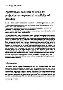
where ∆W1n are independent real Gaussian random variables with mean 0 and varin ance h, and ∆W√ 2 are independent complex Gaussian random variables with mean 0 and variance h/ 2 of both real and imaginary parts. Note that even though we have an exact analytical formula for u2 , we still need to evaluate the stochastic integral in equation (2.4). We perform this evaluation numerically and, therefore, the solution u2 strictly speaking becomes semi-analytical. However, we use a very fine time step of h = 10−3 (which is the same as for the numerical solution) and, therefore, evaluate the integral in equation (2.4) with high precision. The convergence study of the numerical solution that we present below confirms this approximation. In Figure 2.1, we demonstrate both analytical solution (equations (2.3), (2.4)) and numerical approximation (equations (2.15), (2.16)). We note that there is an excellent correspondence between them. Moreover, we observe that for the case of

616

A NONLINEAR TEST MODEL FOR FILTERING SLOW-FAST SYSTEMS (a)

(c) 1

2.5

0.5

2

−0.5

u

1

0 1.5 1

−1 −1.5

0.5 0

0.5

1

1.5

0

5

(b)

15

(d) 1

1

0.5

0.5

0

2

Re[u ]

10

0 −0.5 −0.5

−1

−1

−1.5 0

0.5

1 t

1.5

0

5

10 t

15

Fig. 2.1. The analytical solutions (solid line) are computed via equations (2.3)–(2.4) and the numerical solutions (asterisks) are computed via equations (2.15)–(2.16). Panels (a) and (b) show u1 and Re[u2 ] for the case of strong damping. Panels (c) and (d) show u1 and Re[u2 ] for the case of weak damping. The dashed line represents the exponential decay e−γj t with the corresponding γj for j = {1,2}. Note the different scales of x-axis due to different rates of damping.

strong damping, u2 makes only a few oscillations within its typical decorrelation time (∼ 1/γ2 ), whereas for the case of weak damping, u2 makes many oscillations until it decorrelates. We have confirmed numerically that the Milstein method that we used has the first order convergence with further refinement in h. Next, we compute closed formulas for the mean and covariance of u1 and u2 , which are needed in an extended Kalman filter for the nonlinear system. 2.5. Mean and variance of u1 . equation (2.3), we obtain

We start with u1 . By taking the average of

hu1 i = hu10 ie−γ1 (t−t0 ) ´ ¢ A ³ −γ1 (t−t0 ) ¡ + 2 e ω cos(ωt ) − γ sin(ωt ) − ω cos(ωt) + γ sin(ωt) , 0 1 0 1 γ1 + ω 2 (2.17) where we used the fact that the mean of the stochastic integral is always zero [12]. Furthermore, the variance of u1 becomes Var(u1 ) = h(u1 − hu1 i)2 i = Var(u10 )e−2γ1 (t−t0 ) +

σ12 (1 − e−2γ1 (t−t0 ) ). 2γ1

(2.18)


617

In order to compute the variance we used the Ito isometry formula [12] ¿³ Z ´2 À Z g(t)dW (t) = g 2 (t)dt,

for any deterministic g(t).

2.6. Mean and covariance of u2 .

After averaging equation (2.4), we have

hu2 i = e−γ2 (t−t0 ) hψ(t0 ,t) u20 i.

(2.19)

For simplicity of notation we drop parameters in the functions J(s,t), JD (s,t), JW (s,t), b(s,t), ψ(s,t), ψD (s,t), ψW (s,t) for s = t0 , and denote them as J, JD , JW , b, ψ, ψD , ψW , respectively. Using the assumption that the noise W1 (t) is independent of the initial conditions u10 and u20 , we obtain hu2 i = e−γ2 (t−t0 ) ψD hψW ihu20 exp(ibu10 )i.

(2.20)

The averages in the right hand side of equation (2.20) can be computed via the characteristic function of a Gaussian random variable. For any probability distribution, we define a characteristic function as φv (s) = hexp(isT v)i,

(2.21)

where s ∈ Cd and d is the number of dimensions. For a Gaussian distribution, the characteristic function is known [12] to have the following form: ¶ µ 1 T T (2.22) φv (s) = exp is hvi − s Σs , 2 where Σ is the covariance matrix. In particular, for hψW i we obtain ¶ µ ¶ µ 1 1 iJW i = exp ihJW i − Var(JW ) = exp − Var(JW ) . hψW i = he 2 2

(2.23)

Computation of Var(JW ) is straightforward since JW is Gaussian, and the result is Var(JW ) = −

¢ σ12 a20 ¡ 3 − 4e−γ1 (t−t0 ) + e−2γ1 (t−t0 ) − 2γ1 (t − t0 ) . 2γ13

(2.24)

Next, we compute hu20 exp(ibu10 )i. Here, it is convenient to use the triad real-valued representation of (u1 (t),u2 (t)), x = u1 , y = Re[u2 ],

(2.25) (2.26)

z = Im[u2 ].

(2.27)

Then we just need to find hy0 exp(ibx0 )i and hz0 exp(ibx0 )i, and afterwards combine them using u20 = y0 + iz0 (where the zero subscript refers to the initial values at t = t0 ) to obtain the second average in the right hand side of equation (2.19). Consider a three-dimensional vector v = (x0 ,y0 ,z0 ) and the corresponding characteristic function given by equation (2.22). By its definition, the characteristic function is a Fourier transform of the corresponding probability density function (pdf) Z 1 φv (s) = exp(isT v)g(v)dv. (2.28) (2π)3

618


Next, we use the basic property of Fourier transform, i.e., multiplication by a variable in physical space (e.g., y0 ) corresponds to differentiation over the dual variable (e.g., s2 ). We have Z 1 ∂φv (s) iy0 exp(isT v)g(v)dv = ihy0 exp(isT v)i. (2.29) = ∂s2 (2π)3 Therefore, we obtain

Similarly, we find

¯ ∂φv (s) ¯¯ hy0 exp(ibx0 )i = −i ¯ ∂s2 ¯ ¯ ∂φv (s) ¯¯ hz0 exp(ibx0 )i = −i ¯ ∂s3 ¯

.

(2.30)

s=(b,0,0)T

. s=(b,0,0)T

Using the particular form of a Gaussian pdf for v, we find that ´ ∂φv (s) ³ = ihy0 i − Var(y0 )s2 − Cov(x0 ,y0 )s1 − Cov(y0 ,z0 )s3 φv (s), ∂s2 ´ ∂φv (s) ³ = ihz0 i − Var(z0 )s3 − Cov(x0 ,z0 )s1 − Cov(y0 ,z0 )s2 φv (s). ∂s3

After evaluating the partial derivatives at s = (b,0,0)T , we obtain ¶ µ ³ ´ 1 2 hy0 exp(ibx0 )i = hy0 i + iCov(x0 ,y0 )b exp ibhx0 i − Var(x0 )b , 2 ¶ µ ³ ´ 1 2 hz0 exp(ibx0 )i = hz0 i + iCov(x0 ,z0 )b exp ibhx0 i − Var(x0 )b . 2

(2.31) (2.32)

Combining equations (2.31) and (2.32) yields µ ¶ ³ ´ 1 hu20 exp(ibu10 )i = hu20 i + iCov(u20 ,u10 )b exp ibhu10 i − b2 Var(u10 ) . (2.33) 2

Therefore, we have found all the components of the right hand side of equation (2.20) using the initial data. In a similar manner, we find the variance of u2 , cross-covariance of u2 with u∗2 and of u2 with u1 . We have ³ ´ σ2 ³ ´ Var(u2 ) = e−2γ2 (t−t0 ) Var(u20 ) + |hu20 i|2 − |hu20 ψi|2 ) + 2 1 − e−2γ2 (t−t0 ) , 2γ2 (2.34) where |hu20 ψi|2 = e−Var(JW )−b

2

Var(u10 )

|hu20 i + ibCov(u20 ,u10 )|2 .

(2.35)

In Appendix A, we obtain the cross-covariances in a way similar to computing equation (2.33): ³ ´ Cov(u2 ,u1 ) = ψD hψW ie−(γ1 +γ2 )(t−t0 ) hu10 u20 exp(ibu10 )i − hu10 ihu20 exp(ibu10 )i ´ 1 ∂³ i Var(JW (t0 ,t)) hu20 exp(ibu10 )i, (2.36) + ψD hψW ie−γ2 (t−t0 ) 2 a0 ∂t ∗ Cov(u2 ,u2 ) = exp(−2γ2 (t − t0 ) + 2iJD − 2σJ2W )hu220 exp(i2bu10 )i − hu2 i2 , (2.37)

619


where hu10 u20 exp(ibu10 )i and hu220 exp(i2bu10 )i are given by equations (A.8) and (A.9). 2.7. Testing the analytical formulas via Monte Carlo simulations. It is very instructive to provide a visual comparison of the analytical formulas for the various statistics of u1 and u2 that we derived above with the numerically averaged values using Monte Carlo simulations. We used an ensemble of M = 104 members in Monte Carlo averaging. As an object of study, let us choose the mean of u2 . Strong damping

2

Re[]

0.2 0 −0.2 −0.4 0

0.2

0.4

0.6

0.8

1

1.2

1.4

1.6

1.8

6

7

8

9

Weak damping

0.2

2

Re[]

0.4

0 −0.2 −0.4 −0.6 0

1

2

3

4

5 t

Fig. 2.2. The solid line corresponds to hu2 i, computed via equation (2.20). The circles correspond to Monte Carlo averaging of an ensemble of solutions u2 , each computed via equation (2.4). Note the different scales of x-axis due to different rates of damping.

In Figure 2.2, the solid line represents Re[hu2 i] that we computed via equation (2.20). The circles, on the other hand, were obtained using Monte Carlo averaging of an ensemble of trajectories that were computed via equation (2.4). The upper and lower panels correspond to the case of strong and weak damping, correspondingly. The plots for Im[hu2 i] is not displayed here because they are similar to the plots of Re[hu2 i]. We observe excellent agreement between the analytically obtained mean of u2 and the result of the averaging using Monte Carlo simulation. Next, in Figure 2.3 we demonstrate time evolution of cross-covariance between u2 and u∗2 . Here, we also have very good agreement between the analytical prediction and Monte Carlo averaging. Next, we present the comparison of the analytical formula with the results of Monte Carlo averaging for the correlator hu2 u1 i shown in Figure 2.4. Note that here we again have excellent agreement.

620

A NONLINEAR TEST MODEL FOR FILTERING SLOW-FAST SYSTEMS Strong damping 0.2

2

* 2

Re[Cov(u ,u )]

0.1 0 −0.1 −0.2 0

0.2

0.4

0.6

0.8

1

1.2

1.4

1.6

1.8

6

7

8

9

Weak damping

0.04

2

* 2

Re[Cov(u ,u )]

0.06

0.02 0 −0.02 −0.04 −0.06 0

1

2

3

4

5 t

Fig. 2.3. The solid line corresponds to Cov(u2 ,u∗2 ), computed via equation (2.37). The circles correspond to Monte Carlo averaging of an ensemble of solutions u2 , each computed via equation (2.4). Note the different scales of x-axis due to different rates of damping.

2.8. Nongaussianity of u2 . Here, we present the evidence of nongaussianity of the fast wave u2 with the periodic forcing f1 (t) = Asin(ωt). Due to the nonlinear structure of the governing equation (1.2), it is natural to expect that u2 is not Gaussian. However, as we will see below, depending on the regime of the system we can observe both strongly nongaussian and almost Gaussian statistics of u2 . Note that, as we discussed earlier, the invariant measure of our system is always Gaussian. Therefore, nongaussianity can only appear in the transient. In order to detect the deviation from Gaussian statistics, we measure skewness and kurtosis excess. The skewness and kurtosis are defined as the third and the fourth normalized central moments, correspondingly. For a random variable ξ, the skewness is

skewness =

¿³

´3 À ξ − hξi

,

(2.38)

kurtosis =

¿³

.

(2.39)

Var(ξ)3/2

and kurtosis is ´4 À ξ − hξi

Var(ξ)2

621

BORIS GERSHGORIN AND ANDREW MAJDA Strong damping

2 1

Re[]

0.5

0

−0.5 0

0.2

0.4

0.6

0.8

1

1.2

1.4

1.6

1.8

6

7

8

9

Weak damping

2 1

Re[]

0.5

0

−0.5 0

1

2

3

4

5

Fig. 2.4. The solid line corresponds to hu2 u1 i, computed via equations (2.36), (2.17) and (2.20). The circles correspond to Monte Carlo averaging of an ensemble of solutions u1 , each computed via equation (2.3), and u2 , each computed via equation (2.4). Note the different scales of x-axis due to different rates of damping.

For Gaussian ξ, we obtain skewness = 0 and kurtosis = 3. In general, the skewness and the kurtosis excess, which is equal to kurtosis excess = kurtosis − 3,

(2.40)

measure the nongaussian properties of a given random variable. In Figures 2.5 and 2.6, we demonstrate the time evolution of the skewness and kurtosis excess, respectively, for both the weakly damped and the strongly damped cases. Note that in the strongly damped case (Figures 2.5 and 2.6 upper panels), both skewness and kurtosis excess have values close the Gaussian ones. In the strongly damped case, the transient time is short and the statistics of the system do not deviate much from their Gaussian values. On the other hand, in the weakly damped regime (Figures 2.5 and 2.6 lower panels) we observe strong nongaussianity in both skewness and kurtosis excess. In section 2.3, we have shown that invariant measure for the system (1.1) and (1.2) with f1 (t) ≡ 0 is Gaussian and Figures 2.5 and 2.6 confirm that statistics converge to their Gaussian values after the decorrelation time even for oscillatory f1 (t). We note that a sufficiently large ensemble should be used in Monte Carlo simulations for higher moments in order to obtain a precise result. In our simulation, we used the ensemble of M = 104 members, which is large enough to get an accurate qualitative picture. Finally, we end this section with some comments. In principle, analytic expressions for the higher order moments can be computed in a similar fashion as for the

622


second order statistics; however, the explicit formulas become extremely lengthy. Also, the perceptive reader will note that we could use non-Gaussian initial data in the exact solution for the mean and covariance provided that we know the characteristic function of this random variable explicitly. Strong damping 0.3

Skewness

0.2 0.1 0 −0.1 −0.2 0

0.2

0.4

0.6

0.8

1

1.2

1.4

1.6

1.8

2

6

7

8

9

10

Weak damping 0.3

Skewness

0.2 0.1 0 −0.1 −0.2 0

1

2

3

4

5 t

Fig. 2.5. Skewness evolution for the strongly damped (upper panel) and the weakly damped (lower panel) cases. The weakly damped system is more nongaussian than strongly damped. Note the different scales of x-axis due to different rates of damping.

3. Filtering algorithms for the test model 3.1. Extended Kalman filter. Here, we briefly introduce the extended Kalman filter algorithm for the test model (1.1) and (1.2). Suppose that at time tm = m∆t, where m ≥ 0 is a time step index and ∆t is the observation time step, the truth signal is denoted as um , which is a realization of (u1 ,u2 ) computed via equations (2.3) and (2.4). However, we assume that um is unknown and instead we are given some linear transformation of um distorted by some Gaussian noise 0 vm = Gum + σm ,

(3.1)

where vm is called the observation, G is a rectangular matrix of the size q × 3 with 0 the number of observations q = {1,2,3}, u = (x,y,z)T ≡ (u1 ,Re[u2 ],Im[u2 ])T and σm is the observation noise. The observation noise is assumed to be unbiased (mean-zero) with covariance matrix R0 of the size q × q. The goal of filtering is to find the filtered signal uf , which is as close as possible to the original truth signal u. The information that can be used in filtering is limited to

623

BORIS GERSHGORIN AND ANDREW MAJDA Strong damping

Kurtosis excess

0.2

0

−0.2

−0.4

0

0.2

0.4

0.6

0.8

1

1.2

1.4

1.6

1.8

2

6

7

8

9

10

Weak damping

Kurtosis excess

0.2

0

−0.2

−0.4

0

1

2

3

4

5 t

Fig. 2.6. Kurtosis excess evolution for the strongly damped (upper panel) and the weakly damped (lower panel) cases. The weakly damped system is more nongaussian than strongly damped. Note the different scales of x-axis due to different rates of damping.

• the model for dynamical evolution of um , • the matrix G, 0 • and the mean and covariance of the Gaussian noise σm .

In the case when the evolution of um is described by a linear equation, the best approximation to the truth signal in the least squares sense is given via the Kalman filter algorithm [1, 5]. The Kalman filter consists of two steps: (i) forecasting using the dynamics and (ii) correction using observations. If we assume Gaussian initial conditions, then due to linear dynamics the solution stays linear for all times and can be fully described by the mean and covariance matrix. Denote the mean and covariance of the filtered signal at time tm as huim|m and Γm|m , respectively. Then the forecasting step gives us the following, so called prior, values of the mean and covariance at the next time step tm+1 huim|m → huim+1|m , Γm|m → Γm+1|m .

(3.2)

Note that huim+1|m and Γm+1|m depend solely on the prior information up to time tm . In order to utilize the observations vm+1 at time tm+1 , the least squares correction

624


method is used, which yields the posterior values of mean and covariance huim+1|m+1 = huim+1|m + Km+1 (hvim+1 − Ghuim+1|m ), Γm+1|m+1 = (I3 − Km+1 G)Γm+1|m ,

Km+1 = Γm+1|m GT (GΓm+1|m GT + R0 )−1 ,

(3.3)

where Km+1 is a Kalman gain matrix of the size 3 × q and I3 is the identity 3 × 3 matrix. The posterior distribution is the Gaussian distribution with the mean and covariance given in equation (3.3). We note that Kalman gain tells us how much weight the filter puts on the observations vs prior forecast. In the more general case, when the dynamics is given by nonlinear equations, the procedure described in equations (3.2) and (3.3) is called Extended Kalman Filter (EKF). Due to nonlinearity, the gaussianity of the signal can be lost and this filter may not be optimal anymore. One of the purposes of this paper is to investigate the skill of the EKF using our test model. The advantage of studying the test model (1.1) and (1.2) is in the fact that exact analytical formulas can be used for the mean and covariance (see section 2) in order to make the prior forecast (3.2). In the EKF, we use exact evolution equations for the mean and, therefore, in the simulation we use the mean value of the observation hvim in the first equation of (3.3). The effect of the observation noise size is accounted for in computing the Kalman gain matrix Km+1 . 3.2. Structure of observations. In a typical slow-fast system such as the shallow water equations, observation of pressure, temperature, and velocity automatically mixes the fast and slow components and can corrupt the filtering of the slow component. Below, we introduce prototype observations with these features. We will consider three different types of observations with the corresponding observation matrices G and covariances R0 • 1 observation ³ G= 1

√1 √1 2 2

´

,

1 v1 = x + √ (y + z) + σ10 , 2 0 0 R = 2r , • 2 observations G=

Ã

1 1

√1 2 √1 2

√1 2 − √12

!

,

( v1 = x + √12 (y + z) + σ10 ,

v2 = x + √12 (y − z) + σ20 , µ 0 ¶ 2r 0 R0 = , 0 2r0


• 3 observations

625

 1 √12 √12 G =  1 √12 − √12  , 1 0 0  1 0  v1 = x + √2 (y + z) + σ1 , v2 = x + √12 (y − z) + σ20 ,   v3 = x + σ30 ,  0  2r 0 0 R0 =  0 2r0 0  . 0 0 r0 

Here, we assumed that the observation noise components σ10 , σ20 , and σ30 are independent mean-zero Gaussian with variances 2r0 , 2r0 , and r0 , respectively. 3.3. Generating the truth signal. We generate the truth signal using the following procedure. We consider any random initial data as discussed in section 2 and obtain a realization of the trajectory (u1 ,u2 ) using the exact solutions given by equations (2.3) and (2.4). Note that u1 can be easily computed since its random part is Gaussian with known statistics. However, u2 is not Gaussian and its random part depends on the evolution of u1 . Therefore, even if we need the true trajectory only at discrete times with a time step ∆t, we still need to compute u1 with a much finer resolution with time step h. This fine trajectory of u1 is then used to compute u2 . 3.4. Linear filter with model error. Now, suppose that the prior forecast um+1|m is made using the linearized version of the analytical equations that we obtained in section 2. We set a0 = 0 in equation (1.2) and thus we introduce model error. In this case, the linearization is made at the climatological mean state. As we have seen from the invariant measure, in the long run the correlation between the slow wave u1 and fast wave u2 vanishes and so does the effect of nonlinear coupling through a0 . On the other hand, for shorter observation time steps ∆t, the nongaussianity as an effect of nonlinearity can be sufficiently strong (see section 2.8), and the model error can be rather large. The advantage of using a linear model as an approximation of the true dynamics is for practical application. In real physical problems, the true dynamics of the model are often unknown and ensemble approximations to the Kalman filter are very expensive for a large dimensional system. Thus, the performance of the linear filter in the nonlinear test model for the slow-fast system is interesting for several reasons [15, 16]. Note that the truth signal is always produced via the nonlinear version of equations (1.1) and (1.2) with a0 6= 0. Therefore, if we use the linear approximation to the original system, we may not obtain the optimal filtered signal due to model error. Below, we will compare the error in filtering the test problem using the perfect model assumption (forecast via first two moments for the nonlinear equation) and the linear dynamics equations with model error. In our test model, linearization only affects the fast mode u2 . Substituting a0 = 0 into equation (2.20) yields the following linear Equ. ³ ´ hu2 i = exp (−γ2 + iω0 /ε)∆t hu20 i. (3.4) Therefore, the forecast is made according to

huim+1|m = Bhuim|m + C,

(3.5)

626


where  e−γ1 ∆t 0 0 e−γ2 ∆t cos(α) −e−γ2 ∆t sin(α)  , B = 0 0 e−γ2 ∆t sin(α) e−γ2 ∆t cos(α) 

with

(3.6)

α = ∆tω0 /ε, and 

 F1 (t) C =  0 . 0

(3.7)

equation (3.5) is used as a prior forecast for the mean. Similarly by substituting a0 = 0 into equations (2.34), (2.36), and (2.37) we obtain the prior covariance of the linearized model. 3.4.1. Observability. Another advantage of using linearized equations is that it then becomes possible to strictly address the issue of observability [1, 5]. Let us study the observability of the system for the case of observation type 1. In this case, the observability matrix is defined by   G O =  GB  GB 2   √ √ 1 1/ 2 1/ 2 ³ ´ ³ ´  −γ1 ∆t e−γ  2 ∆t 2 ∆t e−γ √ √ cos(α) + sin(α) cos(α) − sin(α)  , (3.8) e = 2 2 ³  ³ ´ ´ e−2γ1 ∆t

2 ∆t e−2γ √ 2

cos(2α) + sin(2α)

2 ∆t e−2γ √ 2

cos(2α) − sin(2α)

This is a 3 × 3 matrix and in order for the system (3.5) to be fully observable, matrix O should have rank 3. It is easy to conclude from equation (3.8) that whenever we have sin(α) = 0 or equivalently ∆t = 2πlε/ω0 ,

(3.9)

for any integer l, the two last columns become equal and, therefore, matrix O becomes singular. This results in losing observability. Let us find the determinant of O ³£ £ ¤´ ¤2 det(O) = −e−γ2 ∆t sin(α) e−γ2 ∆t − e−γ1 ∆t cos(α) + e−2γ1 ∆t 1 − cos2 (α) .

(3.10)

Therefore, in equation (3.9) we have all the values ∆t for which observability is lost. However, practically we still can lack observability even if the matrix O has rank 3, but is close to being singular, which means that det(O) is close to zero. The analysis of observability of the linearized model will also be useful for the nonlinear regime because linear dynamics still plays an important role in the system evolution in the nonlinear regime. In the nonlinear case, we also might expect deteriorating filter performance around the values of ∆t described by equation (3.9).


627

4. Filter performance 4.1. Details of numerical simulation of filtering. We turn to the discussion of the results of the numerical simulation of EKF on our test model (1.1) and (1.2). Here, we describe the parameters that were used in the numerical simulations. The procedure of generating the truth signal was given in section 2. In order to test the filter performance, we compare the truth signal um with the filtered mean huim|m . We also estimate the role of prior forecasts and observations by studying the prior mean huim|m−1 . In order to measure how well the filter reproduces the truth signal (we refer to this property as filter skill), we use root mean square error (RMSE) and cross correlation (XC) between the truth signal and posterior (and sometimes between truth and prior) signals. RMSE is defined via v u N u1 X |zj − wj |2 , (4.1) RMSE(z − w) = t N j=1

where z and w are the complex vectors to be compared and N is the length of each vector. Looking ahead at Figures 4.1-4.4, where we show individual trajectories that are being filtered, the typical amplitude of u is below 2 in magnitude so the RMSE roughly is twice as big as the normalized percentage error in the study below. For real vectors x and y, the XC is defined by PN j=1 xj yj XC(x,y) = qP (4.2) PN 2 . N 2 j=1 yj j=1 xj

For the complex valued vectors z and w, the cross correlation is computed via ´ 1³ XC(z,w) = XC(Re[z],Re[w]) + XC(Im[z],Im[w]) . (4.3) 2

Note that if two signals are close to each other, the RMSE of their difference is then close to zero and their XC is close to one. On the other hand, for two different signals the RMSE diverges from zero and in principle is unbounded and XC approaches zero. In all the simulations we use N = 104 data filtering cycles with the given observation time step ∆t. The type of observation, observation variance r0 , and observation time step ∆t will be varied and specified in each particular situation. Here, we will only discuss the weak damping case since it has more physical importance for filtering slow-fast systems.

4.2. Examples of filtering individual trajectories. Here, we demonstrate how the EKF works on individual trajectories. We chose two values of the observation time step: ∆t = 0.13 and ∆t = 1.43. The first one is considerably smaller than the typical oscillation period T2 = 2πω0 /ε ≈ 0.63 of the fast mode u2 and the second one is larger than T2 . We also chose two values of the observation variance r0 = 0.1 and r0 = 2.0. The first value of r0 is chosen to be smaller than the average energy of each mode E = 1 and the second value is chosen to be larger than E = 1. Therefore, we have four pairs (∆t,r0 ) for which we have studied the performance of the EKF. We have used observations of type 1 in this numerical experiment so that slow and fast modes are mixed in the single observation. The four panels in Figure 4.1 correspond to the four pairs of parameters (∆t,r0 ). In each panel in Figure 4.1, we demonstrate a segment of the truth trajectory u1

628


/ r0 ∆t 0.1 2.0

0.13

1.43

0.988 (0.982) 0.951 (0.945)

0.936 (0.888) 0.855 (0.823)

Table 4.1. EKF performance on u1 : cross correlations XCp (between truth and posterior) and XCf (in the parenthesis, between truth and prior). The segments of the corresponding trajectories are shown in Figure 4.1.

together with the prior forecast and the posterior signal. In Table 4.1, we also show the cross correlation XCf between the truth signal and prior forecast and cross correlation XCp between the truth signal and posterior signal. Table 4.1 is made for the same set of parameters as Figure 4.1, and the cross correlations were measured along the trajectories of n = 104 observation time steps ∆t. Note that for all four cases we have XCf < XCp , which means that the correction step of the EKF improves the forecast using observations. Comparing the columns of Table 4.1, we observe that the skill of the EKF decreases significantly when we increase ∆t. On the other hand, comparing the rows of Table 4.1, we also observe that the skill of the EKF decreases significantly when we increase r0 . 0

0

(a) ∆t=0.13 r =0.1

(b) ∆t=1.43 r =0.1

1

2 1.5

1

1

0

0.5

u

u

1

0.5

0 −0.5

−0.5

−1 −1 200

201

202

−1.5 200

203

0

210

220

230

0

(c) ∆t=0.13 r =2.0

(d) ∆t=1.43 r =2.0

1

2 1.5

1

1

0

0.5

u

u

1

0.5

0 −0.5

−0.5

−1 −1 200

201

202 t

203

−1.5 200

210

220

230

t

Fig. 4.1. The truth signal u1 is shown with the solid line, the prior forecast is shown with pluses connected with a dotted line, and the posterior signal is shown with circles. The values of ∆t and r 0 are shown on top of each panel. The corresponding cross correlations XCf and XCp are given in Table 4.1. Note the different time scales for different ∆t.

Figure 4.2 shows the evolution of u2 together with the prior forecast and posterior

629

BORIS GERSHGORIN AND ANDREW MAJDA (a) ∆t=0.13 r0=0.1

(b) ∆t=1.43 r0=0.1

1

3 2

2

Re[u ]

2

Re[u ]

0.5

0

−0.5

−1 200

1 0 −1

201

202

−2 200

203

210

(c) ∆t=0.13 r0=2.0 3 2

2

2

Re[u ]

0.5 Re[u ]

230

(d) ∆t=1.43 r0=2.0

1

0

−0.5

−1 200

220

1 0 −1

201

202

203

−2 200

210

t

220

230

t

Fig. 4.2. The truth signal u2 is shown with the solid line, the prior forecast is shown with pluses connected with a dotted line, and the posterior signal is shown with circles. The values of ∆t and r 0 are shown on top of each panel. The corresponding cross correlations XCf and XCp are given in Table 4.2. Note the different time scales for different ∆t.

/ r0 ∆t 0.1 2.0

0.13

1.43

0.967 (0.955) 0.911 (0.897)

0.740 (0.544) 0.622 (0.357)

Table 4.2. EKF performance on u2 : cross correlations XCp (between truth and posterior) and XCf (in the parenthesis, between truth and prior). The segments of the corresponding trajectories are shown in Figure 4.2.

signal. Table 4.2 shows the cross correlations XCp and XCf that correspond to the trajectories of u2 (shown partially in Figure 4.2). Here, we also note the decrease in the skill of the EKF if larger ∆t or r0 are used. However, we should point out that if the time step ∆t becomes significantly larger than the oscillation time T2 (in our case ∆t = 1.43 and T2 ≈ 0.63) we observe very poor filter skill in u2 but not in u1 , which is still filtered quite well (compare XCp = 0.855 for u1 in Table 4.1, with XCp = 0.622 for u2 in Table 4.2 for ∆t = 1.43 and r0 = 2.0). In Secs. 4.5 and 4.6, we present a thorough study of how the EKF performance depends on the observation time step ∆t, observation variance r0 , type of observations, and the model that is used for the forecast.

630


/ r0 ∆t 0.1 2.0

0.13

1.43

0.988 (0.985) 0.951 (0.950)

0.936 (0.921) 0.855 (0.856)

Table 4.3. EKF performance on u1 : cross correlations XCp (between truth and posterior without model error, i.e., a0 = 1) and XCme (in the parenthesis, between truth and posterior with model error, i.e., a0 = 0). The segments of the corresponding trajectories are shown in Figure 4.3.

/ r0 ∆t 0.1 2.0

0.13

1.43

0.967 (0.864) 0.911 (0.618)

0.740 (0.543) 0.622 (0.436)

Table 4.4. EKF performance on u2 : cross correlations XCp (between truth and posterior without model error, i.e., a0 = 1) and XCme (in the parenthesis, between truth and posterior with model error, i.e., a0 = 0). The segments of the corresponding trajectories are shown in Figure 4.4.

4.3. Filtering with model error. Here, we discuss how the filter performance changes if we use the linearized model with a0 = 0 as a prior forecast instead of the exact nonlinear model with a0 6= 0. In Figures 4.3 and 4.4, we show segments of the trajectories of the truth signal together with two filtered signals, where one was obtained using the exact model, and another one — using the linearized model. Here, we had the same set of parameters that we used for generating Figures 4.1 and 4.2. Similarly, we constructed Tables 4.3 and 4.4 with the values of the cross-correlation XCp already discussed above and cross correlation XCme between the truth signal and the posterior signal obtained via the linearized model, i.e., with model error. We note that although by setting a0 = 0 we seem to make u1 and u2 decoupled, they still stay coupled through the mixed observations of type 1 or 2. Observations of type 3 make mode u1 independent from mode u2 throughout the filtering process with model error, i.e., with a0 = 0. By comparing the filtered signals with the truth trajectories, we conclude that model error is quite small in the filtering of u1 (Table 4.3) regardless of the size of r0 or ∆t. Observations of type 1 were used here. On the other hand, using the linearized model for the prior forecast drastically affects the performance of filtering u2 — from Table 4.4, we conclude that XCp > XCme for u2 . Below, we will study how model error depends on the type of observations, observation variance, and observation time step. 4.4. Filtering the linear model and the test of observability. In Figure 4.5, we present the results of the numerical filtering of the linearized problem with a0 = 0. In this simulation, the truth signal was also computed via the linearized version of equations (2.3) and (2.4), i.e., with a0 = 0. Therefore, the Kalman filter produces the optimal filtered signal and there is no model error in this simulation. In Figure 4.5(a), we show the dependency of the RMSE on the observation time step ∆t. In Figure 4.5(b), we demonstrate the corresponding dependency of det(O)−1 on ∆t. We note the strong correlation between the two plots. The peaks that were predicted by observability analysis (Figure 4.5(b)) are observed at the same locations on the plot of RMSE of u1 (Figure 4.5(a)). Here, we have taken very small observation variance r0 = 0.002. Thus, we ensure that the filter tends to trust the observations and, therefore, observability becomes crucial. We note that for the fully observable

631

BORIS GERSHGORIN AND ANDREW MAJDA (b) ∆t=1.43 r0=0.1

0.5

1

1

2

0

u

u

1

(a) ∆t=0.13 r0=0.1 1

−0.5

−1 200

0

−1

201

202

−2 200

203

(c) ∆t=0.13 r0=2.0

210

220

230

(d) ∆t=1.43 r0=2.0

1

2 1.5

1

1

0

0.5

u

u

1

0.5

0 −0.5

−0.5

−1 −1 200

201

202 t

203

−1.5 200

210

220

230

t

Fig. 4.3. The truth signal u1 is shown with the solid line, the posterior signal computed via nonlinear forecast is shown with bold dashed line, and the posterior signal computed via linear forecast is shown with the thin dashed line (note that in panel (d) the two dashed lines almost coincide). The corresponding values of ∆t and r 0 are shown on top of each panel. The corresponding cross correlations XCp and XCme are given in Table 4.3. Note the different time scales for different ∆t.

case, i.e., with observations of type 3, there are no peaks at all. In that case, the observation matrix G always has rank 3, regardless of ∆t. However, for observations of types 1 and 2 we clearly see lack of observability around the values of ∆t predicted by equation (3.9). 4.5. Filter performance as a function of observation time step. Next, we study how performance of the EKF depends on the observation time step ∆t under various conditions such as type of observations, observation variance, and the model used in the prior forecast. As we studied above, for the linear model (a0 = 0) the dependence of the EKF performance on ∆t is strongly correlated with observability properties of the EKF. Here, we will see how that result is reflected in filtering the nonlinear model. In Figure 4.6, we show the RMSE of the filtered solution of u1 compared with the truth signal of u1 . We have chosen three fixed values of observation variance: r0 = 0.002, r0 = 0.256, r0 = 2.048 (panels (a), (b), and (c) in Figure 4.6). For each r0 , we consider all three types of observations. Moreover, for each type of observation, we used two models for the prior forecast: the perfect model with a0 = 1 (the same a0 that was used for creating the truth signal), and the linearized model with a0 = 0 (with model error). As a result of this simulation, we draw the following conclusions: 1. The RMSE of u1 approaches some finite value as ∆t increases and r0 is fixed.

632

A NONLINEAR TEST MODEL FOR FILTERING SLOW-FAST SYSTEMS (a) ∆t=0.13 r0=0.1

(b) ∆t=1.43 r0=0.1

1

3 2

2

Re[u ]

2

Re[u ]

0.5

0

−0.5

−1 200

1 0 −1

201

202

−2 200

203

(c) ∆t=0.13 r0=2.0

230

3 2

2

2

Re[u ]

0.5 Re[u ]

220

(d) ∆t=1.43 r0=2.0

1

0

−0.5

−1 200

210

1 0 −1

201

202 t

203

−2 200

210

220

230

t

Fig. 4.4. The truth signal u2 is shown with the solid line, the posterior signal computed via nonlinear forecast is shown with the bold dashed line, and the posterior signal computed via linear forecast is shown with the thin dashed line (note that in panel (d) the two dashed lines almost coincide). The corresponding values of ∆t and r 0 are shown on top of each panel. The corresponding cross correlations XCp and XCme are given in Table 4.4. Note the different time scales for different ∆t.

2. For observations of types 1 and 2, the EKF performance becomes very poor around the values of ∆t, where the linearized system has lack of observability, whereas observations of type 3 make the EKF always fully observable. 3. A larger number of observations leads to better EKF performance regardless of r0 . 4. For observations of type 3, the RMSE is almost negligible for small r0 and monotonically increases for larger r0 . 5. The model error is much larger with smaller r0 and it becomes almost negligible for larger r0 as ∆t increases. 6. For larger r0 , the peaks that correspond to poor filter performance are less sharp than for smaller r0 , which is explained by the fact that observability is less important with a larger observation error than with a smaller one since greater weight is given to the dynamics. We now study the dependence of the EKF performance on mode u2 , which is shown in Figure 4.7. We make the following observations after examining Figure 4.7: 1. The RMSE of u2 approaches some finite value as ∆t increases and r0 is fixed.

633

BORIS GERSHGORIN AND ANDREW MAJDA (a) 0.5 0.45

obs type 1 obs type 2 obs type 3

0.4

0.3

1

RMSE(u )

0.35

0.25 0.2 0.15 0.1 0.05 0

0.2

0.4

0.6

0.8

1 (b)

1.2

1.4

1.6

1.8

2

0.2

0.4

0.6

0.8

1 ∆t

1.2

1.4

1.6

1.8

2

5

det(O)

−1

10

0

10

Fig. 4.5. (a) The RMSE of u1 for three types of observations and observation variance r 0 = 0.002 as a function of ∆t, (b) det(O)−1 as a function of ∆t (note the logarithmic scale of the y-axis). Weak damping was used.

2. The RMSE of u2 is smaller when the number of observations is larger. 3. Observations of type 1 and 2 show lack of observability at the values of ∆t predicted by observability analysis (equation (3.9)). 4. Observations of type 1 and 2 have an extra peak at ∆t ≈ T2 /2, which also corresponds to lack of observability at this time step (see a small peak at ∆t ≈ T2 /2 in Figure 4.5(b)). This peak was absent in the corresponding plot for u1 . 5. For all ∆t, the difference among the types of observations becomes smaller as r0 increases. 6. For all ∆t, the model error becomes smaller as r0 increases. 4.6. Filter performance as a function of observation variance. In this Section, we study how the filter performance depends on r0 for the fixed observation type and ∆t. In Figure 4.8, we demonstrate the RMSE of filtering u1 as a function of r0 for three different values of ∆t. Let us point out the conclusions that we draw from Figure 4.8: 1. The RMSE is a monotonically growing function of r0 . 2. A larger number of observations lead to better EKF performance regardless of ∆t. 3. In the limit r0 → 0, the RMSE of filtering with observations of types 1 and 2

634

A NONLINEAR TEST MODEL FOR FILTERING SLOW-FAST SYSTEMS (a) r0=0.002

RMSE(u1)

0.6 0.4 0.2 0

0

0.5

1

1.5

2

2.5

3

3.5

4

4.5

5

3

3.5

4

4.5

5

0

(b) r =0.256

RMSE(u1)

0.6 0.4 0.2 0

0

0.5

1

1.5

2

2.5 0

(c) r =2.048

RMSE(u1)

0.6 0.4 0.2 1 0

0

0.5

1

1.5

2 2

3 2.5 ∆t

1 ME 3

3.5

2 ME 4

3 ME 4.5

5

Fig. 4.6. The RMSE of u1 as a function of ∆t. Observations of type 1 (solid line), type 2 (dashed line), and type 3 (dashed-dotted line) with the nonlinear model (bold line) and the linearized model with model error (ME, thin line) were used in the simulation. A fixed r0 (shown on top of the corresponding panel) was used in each simulation.

converges to some finite positive value, which means that even if the observation error is negligible, the filter still does not reproduce the truth signal because the observations of type 1 and 2 only carry partial information about the truth signal. 4. Observations of type 3 lead to a vanishing error as r0 → 0.

5. As r0 grows, the difference in the RMSE for different observation types decreases. This is explained by the fact that EKF chooses to trust the dynamics more when the observation error variance is large and, hence, the influence of the observations on the filtered signal diminishes.

6. The RMSE for filtering with model error (a0 = 0) increases as r0 → 0 for ∆t = 0.63 and observations of types 1 and 2 (thin solid and dashed lines in Figure 4.8(b)). For other values of ∆t (for which the corresponding linear system is observable), the RMSE of filtering with model error is a monotonically decreasing function of r0 . 7. For observations of types 1 and 2, model error due to linearization (difference between the thick and thin solid (observations of type 1) and dashed (observations of type 2) curves) is increasing as r0 → 0. This indicates that the model error increases as r0 approaches 0. We will have a more thorough study of the model error in section 4.7.

635

BORIS GERSHGORIN AND ANDREW MAJDA (a) r0=0.002

RMSE(u2)

1

0.5

0

0

0.5

1

1.5

2

2.5

3

3.5

4

4.5

5

3

3.5

4

4.5

5

0

(b) r =0.256

RMSE(u2)

1

0.5

0

0

0.5

1

1.5

2

2.5 0

(c) r =2.048

RMSE(u2)

1

0.5 1 0

0

0.5

1

1.5

2 2

3 2.5 ∆t

1 ME 3

3.5

2 ME 4

3 ME 4.5

5

Fig. 4.7. The RMSE of u2 as a function of ∆t. Observations of type 1 (solid line), type 2 (dashed line), and type 3 (dashed-dotted line) with the nonlinear model (bold line) and the linearized model with model error (ME, thin line) were used in the simulation. A fixed r0 (shown on top of the corresponding panel) was used in each simulation.

8. The model error is very small with observations of type 3 (thick and thin dashed-dotted lines in Figure 4.8 almost coincide.) Next, we note that the RMSE of u2 as a function of r0 , shown in Figure 4.9, behaves similarly to the RMSE of u1 . However, the error in filtering the fast mode u2 is larger because the faster mode has more irregular time dynamics, which is harder to capture from the observations with finite step ∆t. Moreover, the linearization (a0 = 0) introduces a larger model error in the dynamics of u2 , since for u2 the dynamical equation explicitly depends on a0 , unlike for u1 , where the dependence on a0 only implicitly comes from observations. 4.7. Statistics of mean model error and individual realizations. Mean model error statistics are a standard part of offline testing for Kalman filter performance in linear models [1]. How useful are mean model error statistics as a qualitative guideline for filter performance in nonlinear slow-fast systems? The exact solution formulas for statistics in the test model allow us to address these issues here. Let us now study the mean model error due to linearization. In section 3.4, we estimated model error by following individual trajectories for a given observation type and the set of parameters ∆t and r0 , and then by measuring averaged model error along these trajectories. Now, we consider averaging over all possible ensembles of the random signal trajectories as well as the random noise in observations. This way, we will obtain a fully

636

A NONLINEAR TEST MODEL FOR FILTERING SLOW-FAST SYSTEMS (a) ∆t=0.13

RMSE(u1)

0.6

1

2

3

0.2

0.4

0.6

1 ME

2 ME

3 ME

0.4 0.2 0

0

0.8

1

1.2

1.4

1.6

1.8

2

1.2

1.4

1.6

1.8

2

1.2

1.4

1.6

1.8

2

(b) ∆t=0.63

RMSE(u1)

0.6 0.4 0.2 0

0

0.2

0.4

0.6

0.8

1 (c) ∆t=5.03

RMSE(u1)

0.6 0.4 0.2 0

0

0.2

0.4

0.6

0.8

1 r0

Fig. 4.8. The RMSE of u1 as a function of r 0 . Observations of type 1 (solid line), type 2 (dashed line), and type 3 (dashed-dotted line) with the nonlinear model (bold line) and the linearized model with model error (ME, thin line) were used in the simulation. A fixed ∆t (shown on top of the corresponding panel) was used in each simulation.

deterministic system for estimating mean model error. The solution of this system requires much less computational work than resolving a long individual trajectory and then filtering it. As a result of the mean model error analysis, we expect to obtain some indications of the model error along the individual trajectories. Next, we describe the algorithm of measuring the mean model error. Note that since we have the exact analytical formulas for the time evolution of the mean hui of the model in a nonlinear regime (a0 6= 0), we can compute it, and, therefore, obtain the truth signal for the mean. Moreover, we use the same formulas for hui together with the formulas for the evolution of the covariance but in the linearized form (a0 = 0) to produce a prior forecast. a =0

0 ¯ m|m −− ¯ m+1|m , u −→ u

(4.4)

¯ instead of hui to distinguish between the filtering of where we use the notation u the mean signal and filtering of the individual random trajectories. The posterior forecast in the mean model error estimation is made via the following reasoning. The observations vm = Gum have mean zero, therefore after averaging over all possible

637

BORIS GERSHGORIN AND ANDREW MAJDA (a) ∆t=0.13

RMSE(u2)

1

1

2

3

0.2

0.4

0.6

1 ME

2 ME

3 ME

0.5

0

0

0.8

1

1.2

1.4

1.6

1.8

2

1.2

1.4

1.6

1.8

2

1.2

1.4

1.6

1.8

2

(b) ∆t=0.63

RMSE(u2)

1

0.5

0

0

0.2

0.4

0.6

0.8

1 (c) ∆t=5.03

RMSE(u2)

1

0.5

0

0

0.2

0.4

0.6

0.8

1 r0

Fig. 4.9. The RMSE of u2 as a function of ∆t. Observations of type 1 (solid line), type 2 (dashed line), and type 3 (dashed-dotted line) with the nonlinear model (bold line) and the linearized model with model error (ME, thin line) were used in the simulation. A fixed ∆t (shown on top of the corresponding panel) was used in each simulation.

¯ m = G¯ trajectories we have v um . The correction step of the filter becomes ¯ m+1|m+1 = u ¯ m+1|m + Km+1 G(¯ ¯ m+1|m ), u um+1 − u Γm+1|m+1 = (I3 − Km+1 G)Γm+1|m , Km+1 = Γm+1|m GT (GΓm+1|m GT + R0 )−1 .

(4.5) (4.6) (4.7)

Note that the so-called off-line statistics Γ and K are computed by the same formulas as for the individual trajectories, and only the update of the mean is different. It is necessary to stress here that even though the Kalman filter algorithm for computing the mean model error seems to be the same as for computing the filtered signal of individual trajectories, in the mean model error analysis we do averaging prior to filtering while previously, in the filtering the individual trajectories, we first performed filtering and then did averaging. In Figure 4.10, we demonstrate the time evolution of the mean (panels (a) and (b)) and the covariance (panels (c)-(f)) of (¯ u1 , u ¯2 ) and their corresponding filtered values. Observations of type 1 were used. From Figure 4.10(a), we see that the error in filtering u ¯1 is very small. On the other hand, the error in filtering u ¯2 is rather large within the decorrelation time (∼ 1/γ1 ≈ 1/γ2 ) until both the truth signal u ¯2,m and the filtered signal u ¯2,m|m converge to zero. The mean model error is characterized by the measure of the difference between u ¯m and u ¯m|m , e.g., the cross covariance between

638

A NONLINEAR TEST MODEL FOR FILTERING SLOW-FAST SYSTEMS (a) u ¯1

(b) Re(¯ u2 ) 0.1

1 0

0.5 0

−0.1

exact u ¯m filtered u ¯m |m

−0.5 −0.2 0

10

20

30

40

0

10

(c) V ar(¯ u1 )

20

30

40

(d) V ar(¯ u2 )

0.4

0.8

0.3

0.6

0.2

0.4 0.2

0.1 0

10

20

30

40

0

10

(e) Cov(¯ u2 , u ¯∗2 )

0.03

20

30

40

(f) Cov(¯ u1 , u ¯2 ) 0.02

0.02

0

0.01 −0.02 0 −0.04 0

10

20

30 time

40

0

10

20

30

40

time

Fig. 4.10. Mean model error. The solid line shows the truth values and the circles show the filtered values. r0 = 2.048, ∆t = 2, and observations of type 1 were used.

the two of them. The various components of the truth covariance and posterior covariance reach constant values within the decorrelation time. The difference between the corresponding components of the truth and posterior covariance can be another characteristic of the mean model error. Next, we study what information about the mean model error is relevant to estimating the model error in filtering individual trajectories, and what information can be misleading. In Figure 4.11, we show the dependence of mean model error of the slow mode u1 on the observation time step ∆t for three fixed values observation variance r0 . As a measure of the mean model error, we have chosen the cross-correlation XCM ¯1,m and u ¯1,m|m along the typical decorrelation time (chosen to be 1 between u τ = 30 from studying Figure 4.10, as it appears to be the typical relaxation time). On the other hand, in Figure 4.12, we demonstrate the cross correlation XC1 between the two signals hu1,m|m i filtered from the same individual trajectory: one computed via the nonlinear dynamics (a0 6= 0) and the other one computed via the linearized dynamics (a0 = 0). Moreover, in Figures 4.11 and 4.14, we show similar dependencies of XCM 2 and XC2 on ∆t for the fast mode u2 . It is very instructive to compare Figure 4.11 with Figure 4.12 and Figure 4.13 with Fig 4.14. Below, we present the ideas about the model error that we can predict from the mean model error analysis, i.e., the similarities between XCM 1 and XC1 and between XCM 2 and XC2 : 1. The model error is large at the values of ∆t that were predicted by observ-

639


ability analysis. 2. The model error of filtering with observations of type 3 is much less that with observations of type 1 and 2. 3. For larger r0 , model error is less dependent on the type of observations. 4. Disregarding local oscillations, the model error for u2 first increases as ∆t increases and then decreases. This does not mean that the filter skill improves as ∆t increases, it just means that model error due to linearization becomes less important. 5. For larger r0 , observations of types 2 and 3 give almost same model error, while observations of type 1 lead to larger model error. Now, we point out the properties of the model error along individual trajectories that are not predicted by the mean model error analysis 1. For smaller r0 , observations of type 2 have larger model error than observations of type 1. 2. The measure of the model error is not predicted well quantitatively, although the qualitative behavior is similar. 3. The dependence on ∆t appears to be quite smooth (especially for observations of types 2 and 3), while the mean model error analysis predicts it to be more oscillatory. (a) r0=0.002 1 XCM 1

0.999 0.998 0.997 obs 1

0.996 0.5

1

1.5

2

2.5

obs 2

obs 3

3

3.5

4

4.5

5

3

3.5

4

4.5

5

3

3.5

4

4.5

5

0

(b) r =0.256

XCM 1

1 0.999 0.998 0.5

1

1.5

2

2.5 0

(c) r =2.048

XCM 1

1 0.9998 0.9996 0.9994 0.5

1

1.5

2

2.5 ∆t

Fig. 4.11. Mean model error of u1 . Observations of type 1 (solid line), type 2 (dashed line), and type 3 (dashed-dotted line) are shown.

What is particularly striking here is the strong correlation of the mean model error for the fast mode u2 , from Figure 4.13, with observations of types 1 and 2 (the

640

A NONLINEAR TEST MODEL FOR FILTERING SLOW-FAST SYSTEMS 0

(a) r =0.002

XC

1

1 0.95 0.9 0.5

1

1.5

2

2.5

3

3.5

4

4.5

5

3

3.5

4

4.5

5

3

3.5

(b) r0=0.256 1

XC

1

0.99 0.98 0.97 0.5

1

1.5

2

2.5 0

(c) r =2.048

XC1

1 0.998 0.996 1

0.994 0.5

1

1.5

2

2.5 ∆t

2 4

4.5

3 5

Fig. 4.12. Model error of u1 . Observations of type 1 (solid line), type 2 (dashed line), and type 3 (dashed-dotted line) are shown.

two larger observational noises) with the non-Gaussianity in the truth signal displayed in Figures 2.5 and 2.6. With larger observational noise, the Kalman filter trusts the Gaussian dynamics of the linearized model significantly, so there are larger mean model errors on the faster mode, even with three observations here. Next, we study if the dependence of the mean model error on r0 can provide any guidelines about the model error of the individual trajectories. We compare Figure 4.15 with Figure 4.16 for u1 and Figure 4.17 with Figure 4.18 for u2 . Here, we outline the properties of the model error that follow from the mean model error analysis. 1. The model error of u1 decreases as r0 increases except for very small r0 and observations of type 3, where the model error vanishes as r0 → 0.

2. Observations of type 3 have the smallest model error in u1 .

3. The model error of u2 grows as r0 increases (note opposite behavior for u1 ). 4. The model error becomes independent of the observation type as both ∆t and r0 increase. On the other hand, we note that there are a few facts about the model error that are not reflected in mean model error analysis 1. For small ∆t = 0.13, observations of type 1 show better filtering skill than observations of type 2 for r0 greater than some value (compare the solid and dashed lines in Figure 4.16(a)) (r0 > 0.7.) 2. For bigger ∆t = 0.63, observations of type 1 show better filtering skill than observations of type 2 for r0 smaller than some value (compare the solid and

641

BORIS GERSHGORIN AND ANDREW MAJDA (a) r0=0.002

2

XCM

1

0.5

0

0.5

1

1.5

2

2.5

3

3.5

4

4.5

5

3

3.5

4

4.5

5

4

4.5

5

0

(b) r =0.256

2

XCM

1

0.5

0

0.5

1

1.5

2

2.5 (c) r0=2.048

obs 1

obs 2

obs 3

2

XCM

1

0.5

0

0.5

1

1.5

2

2.5 ∆t

3

3.5

Fig. 4.13. Mean model error of u2 . Observations of type 1 (solid line), type 2 (dashed line), and type 3 (dashed-dotted line) are shown.

dashed lines in Figure 4.16(b)) (r0 < 0.8) 3. The mean model error analysis only provides qualitative estimates about the model error. 5. Concluding discussion In the introduction, we motivated the need to develop a simple nonlinear test model for filtering slow-fast systems and introduced a nonlinear three dimensional real stochastic triad model as the simplest prototype model for slow-fast systems. In section 2, we established analytic non-Gaussian nonlinear statistical properties of the model including exact formulas for the propagating mean and covariance. An exact nonlinear extended Kalman filter (EKF) for the slow-fast system and a linear Kalman filter with a non-trivial model error on the fast dynamics through linearization at the climitological mean state were introduced in section 3. Various aspects of filter performance for these two filters were discussed in section 4. While there were detailed summaries in section 4, it is useful to summarize several features of the filter performance. First, the partial observations of type 1 and 2 were designed to mix both slow and fast modes as occurs in many practical applications. The theoretical analysis of observability in section 3.4.1 lead us to predict deteriorating filter skill in the vicinity of the non-observable times for observations of type 1 and 2 predicted by equation (3.9); this prediction is confirmed for both the linear and nonlinear filters in Figures 4.54.7 for small and moderate observational noise. On the other hand, for observation

642

A NONLINEAR TEST MODEL FOR FILTERING SLOW-FAST SYSTEMS (a) r0=0.002

XC2

1 0.8 0.6 0.5

1

1.5

2

2.5

3

3.5

4

4.5

5

3

3.5

4

4.5

5

0

(b) r =0.256 1

XC2

0.9 0.8 0.7 0.6 0.5

1

1.5

2

2.5 0

(c) r =2.048

XC2

1 0.8 0.6

1 0.5

1

1.5

2

2.5 ∆t

3

3.5

2 4

4.5

3 5

Fig. 4.14. Model error of u2 . Observations of type 1 (solid line), type 2 (dashed line), and type 3 (dashed-dotted line) are shown.

time steps ∆t, which are away from the non-observable ones and either shorter or longer than the fast oscillation period, as reported in section 4.2, the nonlinear EKF always has significant skill on the slow mode u1 for observations of type 1, which mix the slow and fast modes, and retains non-trivial skill for the fast modes (Tables 4.1 and 4.2); on the other hand, the linear filter with model error retains the significant filter skill of the nonlinear model for the slow mode (Table 4.3) but the filter skill for the fast mode deteriorates significantly (Table 4.4). The slow mode in the nonlinear test model has an exact linear slow manifold [27] and the filter skill with model error on the slow mode reflects this fact; nevertheless, these results here suggest interesting possibilities for filtering slow-fast systems by linear systems with model error [15, 16] when only estimates of the slow dynamics are required in an application. Finally, in section 4.7, we compared the exact nonlinear analysis for filtering skill through offline (super)ensemble mean model error in the test model with the actual filter performance for individual realizations discussed throughout the paper, since such offline tests can provide important guidelines for filter performance [1, 22, 4, 14]. It is established in section 4.7 that the offline mean model error analysis for the nonlinear test model provides very good qualitative guidelines for the actual filter performance on individual signals with some discrepancies discussed in detail there. In future work, the authors plan to utilize the nonlinear test model with nontrivial forcing of the fast waves, f2 (t) 6= 0 in equation (1.2), to develop filters with significant skill for both the slow mode and the slow envelope of the fast modes. As noted earlier in the introduction, this is an important problem for filter skill in

643

BORIS GERSHGORIN AND ANDREW MAJDA (a) ∆t=0.13

XCM 1

1 1 0.9999 0.9999 0.9999

obs=1 0.2

0.4

0.6

0.8

1

obs=2

obs=3

1.2

1.4

1.6

1.8

2

1.2

1.4

1.6

1.8

2

1.2

1.4

1.6

1.8

2

(b) ∆t=0.63

XCM 1

0.999 0.998 0.997 0.996 0.2

0.4

0.6

0.8

1 (c) ∆t=5.03

XCM 1

0.9998 0.9996 0.9994 0.9992 0.999 0.2

0.4

0.6

0.8

1 r0

Fig. 4.15. Mean model error of u1 . Observations of type 1 ( solid line), type 2 (dashed line), and type 3 (dashed-dotted line) are shown.

contemporary meteorology where on mesoscales, slow and fast modes are coupled nonlinearly through moist convection [17]. Acknowledgment. The research of A.J. Majda is partially supported by the National Science Foundation grant DMS-0456713, the Office of Naval Research grant N00014-05-1-0164, and the Defense Advanced Research Project Agency grant N0001407-1-0750. B. Gershgorin is supported as a postdoctoral fellow through the last two agencies.

Appendix A. Computation of cross-covariances. In this Appendix, we compute the cross-covariances Cov(u2 ,u∗2 ) and Cov(u2 ,u1 ). For Cov(u2 ,u∗2 ) we find ® Cov(u2 ,u∗2 ) = (u2 − hu2 i)(u2 − hu2 i) = hu22 i − hu2 i2 = e−2γ2 (t−t0 ) hψ 2 u220 i − hu2 i2 , where 2 2 hψ 2 u220 i = ψD hψW ihu220 exp(i2bu10 )i.

(A.1)

644

A NONLINEAR TEST MODEL FOR FILTERING SLOW-FAST SYSTEMS (a) ∆t=0.13

XC1

0.999 0.998 0.997 1

2

3

1.2

1.4

1.6

1.8

2

1.2

1.4

1.6

1.8

2

1.2

1.4

1.6

1.8

2

0.996 0.2

0.4

0.6

0.8

1

XC

1

(b) ∆t=0.63 0.98 0.96 0.94 0.92 0.9 0.2

0.4

0.6

0.8

1 (c) ∆t=5.03

XC1

0.995 0.99 0.985 0.98 0.2

0.4

0.6

0.8

1 r0

Fig. 4.16. Model error of u1 . Observations of type 1 ( solid line), type 2 (dashed line), and type 3 (dashed-dotted line) are shown.

Next, for Cov(u2 ,u1 ) we obtain D E D³ Cov(u2 ,u1 ) = (u2 − hu2 i)(u1 − hu1 i) = e−γ2 (t−t0 ) [ψ(t0 ,t)u20 − hψ(t0 ,t)u20 i] Z t Z t ´E ´³ e−γ1 (t−s) dW1 (s) e−γ2 (t−s) ψ(s,t)dW2 (s) [u10 − hu10 i]e−γ1 (t−t0 ) + σ1 +σ2 t0

t0

= e−(γ1 +γ2 )(t−t0 ) [hu10 u20 ψ(t0 ,t)i − hu10 ihu20 ψ(t0 ,t)i] E DZ t −γ2 (t−t0 ) e−γ1 (t−s) dW1 (s)u20 ψ(t0 ,t) +σ1 e t0

In order to compute the last term, we note that E ∂D exp(iJW (t0 ,t)) ∂t ´E ³ Z t Z s ′ ∂D e−γ1 (s−s ) dW1 (s′ ) ds exp i = σ1 a0 ∂t t0 t0 Z t E D ′ e−γ1 (t−s ) dW1 (s′ ) . = iσ1 a0 exp(iJW (t0 ,t)) t0

On the other hand, we obtain E ´ ³1 ´∂³ ∂D 1 exp(iJW (t0 ,t)) = − exp Var(JW (t0 ,t)) Var(JW (t0 ,t)) . ∂t 2 2 ∂t

645

BORIS GERSHGORIN AND ANDREW MAJDA (a) ∆t=0.13 obs=1

XC

M 2

0.9

obs=2

obs=3

0.8 0.7 0.6 0.5 0.2

0.4

0.6

0.8

1

1.2

1.4

1.6

1.8

2

1.2

1.4

1.6

1.8

2

1.2

1.4

1.6

1.8

2

(b) ∆t=0.63

XC

M 2

0.8 0.6 0.4 0.2 0.2

0.4

0.6

0.8

1

XC

M 2

(c) ∆t=5.03 0.98 0.96 0.94 0.92 0.9 0.88 0.2

0.4

0.6

0.8

1 0 r

Fig. 4.17. Mean model error of u2 . Observations of type 1 ( solid line), type 2 (dashed line), and type 3 (dashed-dotted line) are shown.

Finally, we obtain ³ ´ Cov(u2 ,u1 ) = ψD hψW ie−(γ1 +γ2 )(t−t0 ) hu10 u20 exp(ibu10 )i − hu10 ihu20 exp(ibu10 )i ´ i 1 ∂³ + ψD hψW ie−γ2 (t−t0 ) Var(JW (t0 ,t)) hu20 exp(ibu10 )i. (A.2) 2 a0 ∂t Note that hu20 exp(ibu10 )i is given by equation (2.33). In order to find averages hu220 exp(i2bu10 )i and hu10 u20 exp(ibu10 )i, we use the real representation given by equations (2.25)–(2.27), which reduces the problem to computing the realvalued averages hx0 y0 exp(ibx0 )i, hx0 z0 exp(ibx0 )i, hy02 exp(i2bx0 )i, hz02 exp(i2bx0 )i, hy0 z0 exp(i2bx0 )i. Using the definition of the characteristic function (2.21), we find

646

A NONLINEAR TEST MODEL FOR FILTERING SLOW-FAST SYSTEMS (a) ∆t=0.13 1

2

3

XC

2

0.9 0.8 0.7 0.2

0.4

0.6

0.8

1

1.2

1.4

1.6

1.8

2

1.2

1.4

1.6

1.8

2

1.2

1.4

1.6

1.8

2

(b) ∆t=0.63

XC

2

0.9 0.8 0.7 0.6 0.5 0.2

0.4

0.6

0.8

1 (c) ∆t=5.03

XC

2

0.95 0.9 0.85 0.2

0.4

0.6

0.8

1 r0

Fig. 4.18. Model error of u2 . Observations of type 1 ( solid line), type 2 (dashed line), and type 3 (dashed-dotted line) are shown.

¯ ∂ 2 φv (s) ¯¯ hx0 y0 exp(ibx0 )i = − , ¯ ∂s1 ∂s2 ¯ s=(b,0,0)T ¯ ∂ 2 φv (s) ¯¯ , hx0 z0 exp(ibx0 )i = − ¯ ∂s1 ∂s3 ¯ s=(b,0,0)T ¯ ∂ 2 φv (s) ¯¯ 2 , hy0 exp(i2bx0 )i = − ¯ ∂s22 ¯ s=(2b,0,0)T ¯ ∂ 2 φv (s) ¯¯ 2 hz0 exp(i2bx0 )i = − , ¯ ∂s23 ¯ s=(2b,0,0)T ¯ ∂ 2 φv (s) ¯¯ . hy0 z0 exp(i2bx0 )i = − ¯ ∂s2 ∂s3 ¯ T s=(2b,0,0)

For a Gaussian vector v = (x0 ,y0 ,z0 )T and any complex vector s = (s1 ,s2 ,s3 )T , we have a characteristic function in the form Z φv (s) = exp(isT v)ghvi,Σ (v)dv, (A.3)


647

where mean is given by hvi = (hx0 i,hy0 i,hz0 i)T ,

(A.4)

and covariance matrix is given by   Var(x0 ) Cov(x0 ,y0 ) Cov(x0 ,z0 ) Σ =  Cov(x0 ,y0 ) Var(y0 ) Cov(y0 ,z0 )  . Cov(x0 ,z0 ) Cov(y0 ,z0 ) Var(z0 )

If we expand the inner products, we obtain µ ´¶ 1³ φv (s) = exp i(s1 hx0 i + s2 hy0 i + s3 hz0 i) − Var(x0 )s21 + Var(y0 )s22 + Var(z0 )s23 2 ³ ´ ×exp − Cov(x0 ,y0 )s1 s2 − Cov(x0 ,z0 )s1 s3 − Cov(y0 ,z0 )s2 s3 . (A.5)

After evaluating the partial derivatives of the characteristic function at the prescribed points, we find the following equations

648


´ ³ ∂ 2 φv (s) = −Cov(x0 ,y0 )φv (s) + ihx0 i − Var(x0 )s1 − Cov(x0 ,y0 )s2 − Cov(x0 ,z0 )s3 ∂s1 ∂s2 ³ ´ × ihy0 i − Var(y0 )s2 − Cov(x0 ,y0 )s1 − Cov(y0 ,z0 )s3 φv (s), ³ ´ ∂ 2 φv (s) = −Cov(x0 ,z0 )φv (s) + ihx0 i − Var(x0 )s1 − Cov(x0 ,y0 )s2 − Cov(x0 ,z0 )s3 ∂s1 ∂s3 ´ ³ × ihz0 i − Var(z0 )s3 − Cov(x0 ,z0 )s1 − Cov(y0 ,z0 )s2 φv (s), ! Ã ´2 ³ ∂ 2 φv (s) φv (s), = − Var(y0 ) + ihy0 i − Var(y0 )s2 − Cov(x0 ,y0 )s1 − Cov(y0 ,z0 )s3 ∂s22 ! Ã ´2 ³ ∂ 2 φv (s) φv (s), = − Var(z0 ) + ihz0 i − Var(z0 )s3 − Cov(x0 ,z0 )s1 − Cov(y0 ,z0 )s2 ∂s23 ³ ´ ∂ 2 φv (s) = −Cov(y0 ,z0 )φv (s) + ihy0 i − Var(y0 )s2 − Cov(x0 ,y0 )s1 − Cov(y0 ,z0 )s3 ∂s2 ∂s3 ³ ´ × ihz0 i − Var(z0 )s3 − Cov(x0 ,z0 )s1 − Cov(y0 ,z0 )s2 φv (s),

Finally, we obtain the following averages Ã ! ³ ´³ ´ hx0 y0 exp(ibx0 )i = Cov(x0 ,y0 ) − ihx0 i − Var(x0 )b ihy0 i − Cov(x0 ,y0 )b µ

¶ 1 2 × exp ibhx0 i − Var(x0 )b , 2 Ã ! ³ ´³ ´ hx0 z0 exp(ibx0 )i = Cov(x0 ,z0 ) − ihx0 i − Var(x0 )b ihz0 i − Cov(x0 ,z0 )b ¶ µ 1 × exp ibhx0 i − Var(x0 )b2 , 2 Ã ! ³ ´2 2 hy0 exp(i2bx0 )i = Var(y0 ) − ihy0 i − Cov(x0 ,y0 )2b ¡ ¢ × exp i2bhx0 i − 2Var(x0 )b2 , ! Ã ³ ´2 2 hz0 exp(i2bx0 )i = Var(z0 ) − ihz0 i − Cov(x0 ,z0 )2b

¡ ¢ × exp i2bhx0 i − 2Var(x0 )b2 , Ã ! ³ ´³ ´ hy0 z0 exp(i2bx0 )i = Cov(y0 ,z0 ) − ihy0 i − Cov(x0 ,y0 )2b ihz0 i − Cov(x0 ,z0 )2b ¡ ¢ × exp i2bhx0 i − 2Var(x0 )b2 ,

Next, we use the following properties of the covariances Cov(u2 ,u∗2 ) = Var(y) − Var(z) + 2iCov(y,z), Cov(u2 ,u1 ) = Cov(x,y) + iCov(x,z),

(A.6) (A.7)


649

to obtain hu10 u20 exp(ibu10 )i Ã

³ ´ = hu10 ihu20 i + Cov(u20 ,u10 ) + ib hu10 iCov(u20 ,u10 ) + hu20 iVar(u10 ) !

¶ 1 2 − b Var(u10 )Cov(u20 ,u10 ) exp ibhu10 i − b Var(u10 ) , 2 2

µ

hu220 exp(i2bu10 )i ´ ³ = Cov(u20 ,u∗20 ) + hu20 i2 + 4bihu20 iCov(u20 ,u10 ) − 4b2 Cov(u20 ,u10 )2 ¡ ¢ × exp i2bhu10 i − 2b2 Var(u10 ) .

(A.8)

(A.9)

REFERENCES [1] B.D.O. Anderson and J.B. Moore, Optimal Filtering, Prentice-Hall Englewood Cliffs, NJ, 1979. [2] J.L. Anderson, An ensemble adjustment Kalman filter for data assimilation, Mon. Wea. Rev., 129(12), 2884–2903, 2001. [3] J.L. Anderson, A local least squares framework for ensemble filtering, Mon. Wea. Rev., 131(4), 634–642, 2003. [4] E. Castronovo, J. Harlim and A. Majda, Mathematical criteria for filtering complex systems: plentiful observations, J. Comp. Phys., 227(7), 3678–3714, 2008. [5] C. Chui and G. Chen, Kalman Filtering, Springer New York, 1999. [6] S.E. Cohn and S.F. Parrish, The behavior of forecast error covariances for a Kalman filter in two dimensions, Mon. Wea. Rev., 119, 1757–1785, 1991. [7] R. Daley, Atmospheric Data Analysis, Cambridge University Press, 457, 1991. [8] R. Durrett, Stochastic Calculus: A Practical Introduction, CRC-Press LLC, 1996. [9] P.F. Embid and A.J. Majda, Low Froude number limiting dynamics for stably stratified flow with small or finite Rossby number, Geophys. Astrophys. Fluid Dyn., 87, 1–50, 1998. [10] G. Evensen, Sequential data assimilation with a nonlinear quasigeostrophic model using Monte Carlo methods to forecast error statistics, J. Geophys. Res., 99, 10143–10162, 1994. [11] G. Evensen, Advanced data assimilation for strongly nonlinear dynamics, Mon. Wea. Rev., 125 1342–1354, 1997. [12] C.W. Gardiner, Handbook of Stochastic Methods for Physics, Chemistry, and Natural Sciences, Springer-Verlag, New York, 1997. [13] M. Ghil and P. Malanotte-Rizzoli, Data assimilation in meteorology and oceanography, Adv. in Geophys., 33, 141–266, 1991. [14] J. Harlim and A. Majda, Mathematical strategies for filtering complex systems: regularly spaced sparse observations, J. of Comp. Phys, doi:10.1016/j.jcp2008.01.049, 2008. [15] J. Harlim and A. Majda, Filtering nonlinear dynamical systems with linear stochastic models, Nonlinearity, submitted, 2007. [16] J. Harlim and A. Majda, Catastrophic filter divergence in filtering nonlinear dissipative systems, Commun. Math. Sci., to appear, 2008. [17] R. Klein and A. Majda, Systematic multiscale models for deep convection on mesoscales, Theo. Comp. Fluid Dyn., 20, 525–551, 2006. [18] R. Kubo, Stochastic Liouville equations, J. Math. Phys., 4(2), 174–183, 1963. [19] E.N. Lorenz, Deterministic non-periodic flow, J. Atmos. Sci., 20, 130–141, 1963. [20] E.N. Lorenz, On the existence of a slow manifold, J. Atmos. Sci., 43, 1547–1557, 1986. [21] A. Majda, Introduction to PDEs and Waves for the Atmosphere and Ocean, Volume 9 of Courant Lecture Notes in Mathematics, AIMS/CIMS, New York, 2003. [22] A.J. Majda and M. Grote, Explicit off-line criteria for stable accurate time filtering of strongly unstable spatially extended systems, Proc. Nat. Acad. Sci., 104, 1124–1129, 2007. [23] A.J. Majda and P.R. Kramer, Simplified models for turbulent diffusion: theory, numerical modelling and physical phenomena, Phys. Rep., 314(4–5), 237–574, 1999. [24] A.J. Majda, I. Timofeyev and E. Vanden-Eijnden, A mathematical framework for stochastic climate models, Commun. Pure Appl. Math, 54, 891–974, 2001.

650


[25] A.J. Majda, I. Timofeyev and E. Vanden-Eijnden, A priori tests of a stochastic mode reduction strategy, Physica D, 170, 206–252, 2002. [26] R.N. Miller, E.F. Carter and S.T. Blue, Data assimilation into nonlinear stochastic models, Tellus A, 51(2), 167–194, 1999. [27] L.J. Neef, S.M. Polavarapu and T.G Shepherd, Four-dimensional data assimilation and balanced dynamics, J. Atmos. Sci., 63, 1840–1858, 2006. [28] E. Ott, B. Hunt, I. Szunyogh, A. Zimin, E. Kostelich, M. Corrazza, E. Kalnay and J. Yorke, A local ensemble Kalman filter for atmospheric data assimilation, Tellus A, 56, 415–428, 2004. [29] R. Salmon, Lectures On Geophysical Fluid Dynamics, Oxford university Press, 378, 1998. [30] L.M. Smith, Numerical study of two-dimensional stratified turbulence. Advances in wave interaction and turbulence, Contemp. Math., 283, 2001. [31] L.M. Smith and F. Waleffe, Generation of slow large scales in forced rotating stratified turbulence, J. Fluid Mech., 451, 145–168, 2002. [32] M.L. Waite and P. Bartello, Stratified turbulence dominated by vortical motion, J. Fluid Mech., 517, 281–308, 2004.