The 1D model consists of a linear array of plaquettes, while the 2D and 3D models are based on the square and cubic lattices respectively. In particular, we have ...
Text of an invited talk given at The 8th International Conference on Recent Progress in Many-body Physics 22-27 August 1994, SchloßSeggau, Styria, Austria
arXiv:cond-mat/9411012v1 2 Nov 1994
A NONPERTURBATIVE MICROSCOPIC THEORY OF HAMILTONIAN LATTICE GAUGE SYSTEMS R.F. Bishop, N.J. Davidson, and Y. Xian Department of Mathematics, UMIST (University of Manchester Institute of Science and Technology) P.O. Box 88, Manchester M60 1QD, UK A review is given of our recent application of a systematic microscopic formulation of quantum many-body theory, namely the coupled-cluster method (CCM), to Hamiltonian U (1) lattice gauge models in the pure gauge sector. It is emphasized that our CCM results represent a natural extension or resummation of the results from the strong-coupling perturbation theory.
1
INTRODUCTION
Lattice gauge field theory was first developed by Wilson [1] in Euclidean space-time to tackle the problem of quark confinement for the strong interaction. Independently, the equivalent Hamiltonian models were formulated by Kogut and Susskind [2]. The lattice supplies an ultra-violet cut-off which regularizes the divergency often encountered in continuum field theory. One of the key advantages of lattice gauge theory clearly lies in the fact that the confining strong-coupling limit provides a natural basis from which one can apply such techniques as perturbation theory and other many-body theory approximations. The fact that the physical continuum limit is achieved in the weak-coupling limit provides a stringent test for any technique applied to lattice gauge theory. There is a general theorem which states that all lattice gauge models possess a nonzero confining region in which the strong-coupling perturbation theory is valid [3]. In other words, the strong-coupling perturbation series of all lattice gauge models have a finite radius of convergence. One challenge in lattice gauge theory is to extend the strong-coupling results to the weak-coupling regime. Methods based on Pad´e approximants and similar techniques are often used for this purpose [4]. However, this rather ad hoc approach requires a prior knowledge of the weak-coupling limit. Among many other techniques, including finite size calculations [5], renormalization group methods [6], t-expansion techniques [7], and loop calculus [8] etc., the numerical Monte Carlo simulations [9] seem provide the most reliable results, although the method is computationally intensive in practice. Recently, several attempts have been made to apply powerful many-body theories to Hamiltonian lattice gauge systems. Two such applications include the method of correlated basis functions (CBF) [10] and the coupled-cluster method (CCM) [11, 12], both of which provide intrinsically nonperturbative results. In this article, we review our recent progress in the application of the CCM to the vacuum state of the U (1) lattice gauge theory in 1 + 1, 2 + 1 and 3 + 1 dimensions (referred to as 1D, 2D, and 3D respectively). The 1D model consists of a linear array of plaquettes, while the 2D and 3D models are based on the square and cubic lattices respectively. In particular, we have formulated the lattice gauge Hamiltonian in terms of a many-body theory and applied several well-tested approximation schemes within the framework of the CCM. These approximation schemes of the CCM have been developed by us for quantum spin lattice systems and have met with considerable success [13]. Not only are they able to produce results for quantum spin lattice models with accuracy comparable to that of the best Monte Carlo calculations, but they also enable us to study the possible quantum phase transitions of 1
the systems in a systematic and unbiased manner [14]. This second ability of the CCM may prove especially significant here since lattice gauge systems may experience a deconfining phase transition as the coupling parameter varies from strong to weak. We notice that the 3D U (1) gauge lattice model must recover a deconfined continuum QED in the weak coupling limit. However, it is widely believed that the confining phase persists for all couplings for the U (1) models in 1D and 2D, and for the SU (2) and SU (3) models in less than four spatial dimensions [15]. The rest of our article is organized as follows. In Sec. 2 we first discuss the number of independent degrees of freedom for the U (1) lattice models in the pure gauge sector, and then transform the gauge invariant Hamiltonian into a many-body Hamiltonian. We present the results for the ground-state energy as a function of the coupling parameter for the U (1) models in 1D and 2D in Sec. 3, and the results of the 3D model in Sec. 4. We conclude our article with a discussion in Sec. 5.
2
THE U(1) MODELS AND THEIR DEGREES OF FREEDOM
In lattice gauge models, the physical fields are defined on the directed links {l} of the lattice. In particular, the Abelian U (1) lattice Hamiltonian after suitable scaling can be written as [2, 11] H=
Nl X 1 l=1
2
El2 + λ
Np X p=1
(1 − cos Bp ),
(1)
where the link index l runs over all Nl links of the lattice, the plaquette index p over all Np elementary lattice plaquettes, and λ is the coupling constant, with λ = 0 being referred to as the strong-coupling limit and λ → ∞ as the weak-coupling limit. Clearly, we shall be interested in the bulk (thermodynamic) limit, where Nl , Np → ∞. If Ns is the number of lattice sites, it is easy to see that in the bulk limit we have Nl = 3Np , Ns = 2Np in 1D; Nl = 2Np , Ns = Np in 2D; and Nl = Np , Ns = Np /3 in 3D. The electric field El is defined on the link l, while the magnetic field Bp is a plaquette variable, given by the lattice curl of the link-variable vector potential Al as Bp ≡ Al1 + Al2 − Al3 − Al4 ,
(2)
with the four links, l1 , l2 , l3 and l4 , enclosing an elementary square plaquette p in the counter-clockwise direction. The direction of the magnetic field Bp can be defined by the right-hand rule around the plaquette. The quantization of the fields is given by the commutator, [Al , El′ ] = iδll′ .
(3)
If we choose the representation, El = −i∂/∂Al, the Hamiltonian of Eq. (1) becomes H =−
Np Nl X X 1 ∂2 (1 − cos Bp ), + λ 2 ∂A2l p=1
(4)
l=1
where the compact variable Al is restricted to the region −π < Al ≤ π. The inner product between ˜ states |Ψ({Al })i and |Ψ({A l })i is defined as: ˜ hΨ|Ψi A =
Nl �Z Y l=1
π
−π
dAl 2π
�
˜ ∗ ({Al })Ψ({Al }). Ψ
(5)
It is useful to denote each link l by both a lattice site vector n and an index α indicating direction, α = ±x, ±y, ±z, so that El ≡ Eα (n), for example. By definition, one has E−x (n) = −Ex (n − x ˆ), etc., 2
where x ˆ is a unit lattice vector in the +x-direction. Similar definitions hold for the vector potential Aα (n). The lattice divergence of the electric field on a site n can now be written as X (∇ · E)(n) = Eα (n); (6) α
where the summation is over α = ±x, ±y, ±z. A gauge transformation of any operator, such as the vector potential Ax (n), is given by " N # " # Ns s X X exp i φ(m)(∇ · E)(m) Ax (n) exp −i φ(m)(∇ · E)(m) = Ax (n) + φ(n) − φ(n + x ˆ), (7) m
m
where Ns is the total number of lattice sites and φ(m) is an arbitrary gauge function. Clearly, the plaquette variable Bp is invariant under this gauge transformation according to the definition of Eq. (2). It is also easy to show that the Hamiltonian of Eq. (4) is invariant under this gauge transformation, as expected. One can also define the divergence of the plaquette variable Bp on a lattice site n. Clearly, this divergence is zero in 1D and 2D because the plaquette direction (i.e., unit vector perpendicular to the plaquette with the right-hand rule) is a constant. In 3D, the plaquette direction varies from plaquette to plaquette. We associate an elementary cube with each lattice site n, with n at the origin of the cube in Cartesian coordinates, and denote the six plaquette variables as Bβ (n) with plaquette direction β = ±x, ±y, ±z, where for example, β = z represents the bottom plaquette of the cube, β = −z the top plaquette of the cube, etc. For later purposes, we refer to the three plaquettes Bβ (n) with β = x, y, z as positive plaquettes with respect to the cube at n, and the other three with β = −x, −y, −z as negative. By definition, for the negative plaquette, one has B−z (n) = −Bz (n + zˆ), etc. The divergence of the plaquette variable at lattice site n can then be clearly written as X (∇ · B)(n) = − Bβ (n), (8) β
with summation over β = ±x, ±y, ±z. We notice that upon substitution of Eq. (2), Eq. (8) yields constant zero, as required by the Bianchi identity, namely (∇ · B)(n) = 0,
∀n.
(9)
We now discuss the number of independent degrees of freedom. Since we are working with the pure gauge Hamiltonians, we restrict ourselves to the gauge-invariant (vacuum) sector of Hilbert space. We therefore require that any state |Ψi satisfies (∇ · E)(n)|Ψi = 0,
∀n.
(10)
This imposes Ns restrictions on the Nl vector potential variables {Al }, where Ns is the number of lattice sites. Therefore, the number of independent variables for U (1) lattice models in the vacuum sector is reduced to N = Nl − Ns . We also note that if the wavefunction Ψ is written as a function of plaquette variables, namely Ψ = Ψ({Bp }), Eq. (10) is satisfied. It is easy to see that for the infinite lattice in 1D and 2D, N = Np , namely, the number of independent degrees of freedom is equal to the number of plaquette variables. Therefore, it is proper and convenient to employ the plaquette variables {Bp } for the 1D and 2D models. The corresponding inner ˜ product between two states |Ψ({Bp }i and |Ψ({B p })i is then defined by integrals over all plaquette variables, � Np �Z π Y dBp ˜ ∗ ˜ Ψ ({Bp })Ψ({Bp }). (11) hΨ|Ψi = B −π 2π p=1 3
For the infinite 3D lattice model, however, one has that N = 2Np /3. If one is to employ the plaquette variables {Bp } in taking the inner products as discussed above for the 1D and 2D models, one still has to satisfy the Ns (= Np /3) geometrical constraints of the Bianchi identity, Eq. (9). In general, these restrictions are quite difficult to apply. It is therefore more convenient to employ the Nl (= Np ) link variables {Al } for the 3D model when taking the inner products, as defined by Eq. (5). The gauge invariance constraint of Eq. (10) are then automatically satisfied so long as the wavefunctions are completely expressible in terms of plaquette variables {Bp }. Since we are dealing with compact lattice gauge theory (i.e., −π < Al ≤ π), the redundant degrees of freedom in {Al } have no effect on evaluating expectation values with normalized wavefunctions. The conclusion of the above discussion is that when taking inner products, we shall employ plaquette variables {Bp } for the 1D and 2D models, and employ link variables {Al } for the 3D case; but the wavefunctions of all models should always be expressible in terms of the plaquette variables alone. Therefore, it is convenient to transform the Hamiltonian of Eq. (4) into a form in which only plaquette variables appear. By using the linear relation of Eq. (2), this can be easily done. We thus derive � Np z Np � X 1 XX ∂2 ∂2 ρ , (12) + λ(1 + cos B ) + (−1) −2 H= p ∂Bp2 2 p ρ ∂Bp ∂Bp+ρ p=1 where ρ is the nearest-neighbour plaquette index, the summation over it runs over all z nearestneighbours plaquettes, and where we have employed the notation � 1, ρ ∈ ρk ; (−1)ρ = (13) (−1)ρ⊥ , ρ ∈ ρ⊥ , and (−1)ρ⊥ =
�
1, if p and p + ρ⊥ denote both positive or both negative plaquettes; −1, otherwise.
(14)
In Eqs. (13) and (14), ρk and ρ⊥ denote nearest-neighbour parallel and perpendicular plaquette indices respectively, and the positive or negative plaquettes have been defined in the paragraph before Eq. (8).
3
GROUND-STATE ENERGY FOR THE 1D AND 2D MODELS
As discussed in Sec. 2, the proper variables for the 1D and 2D U (1) models are the plaquette variables {Bp }. The Hamiltonian of Eq. (12), for the 1D and 2D cases, reduces to H=
Np � X p=1
−2
� Np z ∂2 1 XX ∂2 ; + λ(1 − cos B ) + p 2 ∂Bp 2 p=1 ρ ∂Bp ∂Bp+ρ
−π ≤ Bp ≤ π,
(15)
where we have dropped the parallel symbol, ρ = ρk , and z = 2, 4 for the 1D and 2D cases respectively. The details of our calculations for Eq. (15) have been published elsewhere [11]. In particular, we P first consider the independent plaquette Hamiltonian in the strong-coupling limit (λ = 0), H0 = −2 p d2 /dBp2 , which has two sets of eigenstates, namely {cos mB; m = 0, 1, 2, ...} with even parity and {sin mB; m = 1, 2, ...} with odd parity. The corresponding ground state is clearly a constant, which is referred to as the electric vacuum in the literature. We take this electric vacuum state as our CCM model state |Φi. Hence we have, |Φi = C = 1. The many-plaquette exact ground state |Ψg i of the full Hamiltonian is, according to the CCM ansatz, written as |Ψg i = eS |Φi,
S=
Np X
k=1
4
Sk ,
(16)
where the correlation operator S is partitioned into k-plaquette operators {Sk }. For example, the one-plaquette operator is defined as S1 =
Np ∞ X X
n=1 p=1
Sp (n) cos nBp ;
(17)
and the two-plaquette operator consists of two terms, Np
∞
X′ 1 X S2 = 2! n ,n =1 p ,p =1 1
2
1
2
�
(n1 , n2 ) cos n1 Bp1 cos n2 Bp2 Sp(1) 1 p2
� (n1 , n2 ) sin n1 Bp1 sin n2 Bp2 , +Sp(2) 1 p2
(18)
where the prime on the summation excludes the terms with p1 = p2 . We note that the many-plaquette correlation operators Sk have a close relation to the usual Wilson loops [1, 2]. For example, one can write 2 cos B1 cos B2 = cos(B1 + B2 ) + cos(B1 − B2 ), which corresponds to the following relation for the Wilson loops:
Our parametrization exemplified by Eqs. (17) and (18) is clearly complete. It is also particularly useful in view of the orthonormality of the basis. However, for the 3D model, since we have to employ the link variables when taking inner products, this orthonormality is in some sense lost. We shall discuss this point in the next section. From the Schr¨odinger ground-state equation, H|Ψg i = Eg |Ψg i, or e−S HeS |Φi = Eg |Φi, we obtain the equations for the ground-state energy Eg and the correlation coefficients {Sp , Sp1 p2 , · · ·} by taking proper projections. In particular, the energy equation and the one-plaquette equations can be written together as hΦ| cos nBp e−S HeS |ΦiB = Eg δn,0 ; n = 0, 1, 2, ..., (19) and the two-plaquette equations consist of two sets of inner products, hΦ| cos n1 Bp1 cos n2 Bp2 e−S HeS |ΦiB hΦ| sin n1 Bp1 sin n2 Bp2 e
−S
S
He |ΦiB
=
0,
(20)
=
0,
(21)
where n1 , n2 = 1, 2, ... and p1 6= p2 as before. The higher-order equations can be written down in a similar fashion. In Eqs. (19)-(21), the notation h· · ·iB implies that the inner products are integrals over all plaquette variables {Bp }, as defined by Eq. (11). As usual, one needs to employ a truncation scheme for the correlation operator S. We first consider the SUB1 scheme, in which one sets Sk = 0 for all k > 1. After an extension of the definition for the one-plaquette coefficients {Sp (n)} to include the negative modes (negative n), and taking advantage of the lattice translational invariance to introduce the definition, am ≡ mSp (m), Eq. (19) can be readily written as � � ∞ 1 1 X Eg − λ δm,0 + λ(δm,1 + δm,−1 ) − mam − an am−n = 0, (22) Np 2 2 n=−∞
where m may be any integer. We note that the energy equation is given by setting m = 0. Equation (22) can in fact be transformed to the well-known Mathieu equation corresponding to the single-body Schr¨odinger equation with the one-plaquette Hamiltonian given by the first term of Eq. (15) [11]. We solve these SUB1 equations numerically by a hierarchical sub-truncation scheme, the so-called SUB1(n) scheme in which one retains at the nth level of approximation only those coefficients am 5
Figure 1: Ground-state energy per plaquette for the 2D U (1) model on the square lattice in the LSUB2(n) scheme. Also shown are the full SUB1 results and the results from the nth-order strongcoupling perturbation series, PTn.
with |m| ≤ n, and sets the remainder with |m| > n to zero. For example, in the SUB1(1) scheme, a1 is the only retained coefficient. The solution is trivially obtained from Eq. (22) as a1 =
λ , 2
1 Eg = λ − λ2 ; Np 4
SUB1(1).
(23)
This SUB1(1) result is in fact identical to the result obtained from second-order perturbation theory about the strong-coupling (λ → 0) limit. However, the subsequent SUB1(n) approximations with n > 1 give results far superior to those of perturbation theory. A detailed discussion has been given in Ref. [11]. We next discuss the two-plaquette approximation, i.e., the SUB2 scheme in which one makes the substitution S → SSUB2 = S1 + S2 . As defined by Eq. (18), there are two sets of two-plaquette coefficients which are determined by Eqs. (20) and (21) respectively. Together with the one-plaquette equations discussed above, one has three sets of coupled equations. Since the complete SUB2 approximation is very ambitious as a first attempt to include correlations, we employ instead the local approximation developed by us for the spin-lattice models, namely the LSUBm scheme. We consider just the LSUB2 scheme which includes only nearest-neighbour plaquette correlations. Similar to the SUB1(n) scheme discussed above, we may also introduce the so-called LSUB2(n) sub-truncation scheme in terms of the number of modes {nk } kept Pin the sums in Eqs. (17) and (18) by ignoring those terms in the LSUB2 correlation operator with k nk > n. For example, the LSUB2(1) scheme is identical to the SUB1(1) scheme considered previously in which only a single coefficient a1 is retained. In the LSUB2(2) scheme, however, four coefficients are retained, two of them from the one-plaquette correlations, the other two from the two-plaquette correlations. We notice that in the strong-coupling limit (λ → 0) the LSUB2(2) approximation exactly reproduces the results of the corresponding perturbation series up to the fourth order, � 89 Eg λ4 + O(λ6 ), 1D; λ − 41 λ2 + 3840 (24) → 1 2 73 λ − 4 λ + 3840 λ4 + O(λ6 ), 2D. Np The results for the ground-state energy in the LSUB2(n) scheme up to n = 10 are shown as functions of λ in Table 1 and 2 for the 1D and 2D models respectively, together with some results 6
Table 1: Ground-state energy per plaquette at several values of λ for the 1D U(1) model. Shown are the results from the CCM LSUB2(n) calculations, and from the strong- and weak-coupling expansion series, denoted as PTm(S) (mth order) and PT(W) respectively. λ Method
0.5
1
2
3
4
5
6
8
10
SUB1 LSUB2(2) LSUB2(3) LSUB2(4) LSUB2(6) LSUB2(8) LSUB2(10) PT4(S) PT(W)
0.4391 0.4389 0.4389 0.4389 0.4389 0.4389 0.4389 0.4389 0.5744
0.7724 0.7689 0.7703 0.7702 0.7702 0.7702 0.7702 0.7732 0.8624
1.2430 1.1980 1.2319 1.2320 1.2322 1.2322 1.2322 1.3708 1.2697
1.5828 1.3684 1.5567 1.5615 1.5637 1.5637 1.5638 2.6273 1.5822
1.8597 1.1115 1.8019 1.8243 1.8343 1.8345 1.8345 5.9333 1.8457
2.1000 –0.3116 1.9821 2.0409 2.0692 2.0698 2.0700 13.236 2.0778
2.3156 –6.3126 2.1017 2.2184 2.2798 2.2811 2.2815 27.038 2.2877
2.6966
3.0315
2.1670 2.4663 2.6501 2.6540 2.6557 86.933 2.6603
2.0078 2.5844 2.9714 2.9796 2.9841 2.9886
of nth-order strong-coupling perturbation theory, denoted as PTn(S). We note that we have taken this opportunity to correct some minor errors in the values cited previously in Ref. [11]. We also show the results of the 2D case in Fig. 1. The corresponding 1D curves behave similarly. In Table 2 we have also included the results from the method of correlated basis functions (CBF) [10], from an analytical continuation of the strong-coupling perturbation series (HOZ) [4], and from the t-expansion calculation of Morningstar [7]. Our LSUB2(10) results are in good agreement with them. One sees clearly in Fig. 1 that our LSUB2(n) results quickly converge as n increases. It is also clear that the strong-coupling perturbation series gives very poor results for λ ≥ 1.5, a value which seems to be a good estimate for its radius of convergence. Much work in modern quantum field theory goes into attempts to continue analytically such perturbation series as Eq. (24) outside their natural boundaries. A typical recent such attempt [4] for the 2D U (1) model starts from the strong-coupling perturbation series of Eq. (24), utilizing the known coefficients up to O(λ18 ) as input to generalized Pad´e approximants. The results of this approximation are shown in Table 2 where they are labelled as HOZ. We should emphasize that our own LSUB2(n) approximations themselves represent a natural extension of perturbation theory. They may be contrasted with the rather ad hoc approaches based on Pad´e and other resummation techniques, which usually find it difficult to approach the weak-coupling limit with the correct asymptotic form unless this is built in from the start. It is worth mentioning that in quantum chemistry and other many-body systems, the more relevant physical quantity is the so called correlation energy which is defined as the difference between the mean-field one-body (SUB1 in the present case) and the exact ground-state energies. This correlation energy can be measured experimentally in the cases of atoms and molecules. From Table 1 and 2 and Fig. 1, one can see that the correlation energy within the LSUB2 approximation (i.e., the LSUB2 results minus the SUB1 results) in the U (1) model is quite small, and much smaller than the total energy. We suspect that this is true for lattice gauge field theories in general. This is quite similar to the case in quantum chemistry where the correlation energy is typically only a few percent at most of the total energy. It is clear that a powerful many-body technique is required in order to obtain a sensible numerical value for this correlation energy. The perturbation series in the weak-coupling limit (λ → ∞) is given by √ 1 Eg → C0 λ − C02 + O(λ−1/2 ), Np 8
(25)
where C0 = 1, 0.9833, 0.9581 in 0D (i.e., one-plaquette or Mathieu problem), 1D and 2D respectively. We also show the results from this weak-coupling series in Table 1 and 2, denoted as PT(W). Although our LSUB2(n) schemes do not produce exactly these numbers, they do give good results even for very 7
Table 2: Ground-state energy per plaquette at several values of λ for the 2D U(1) model. Shown are the results from the CCM LSUB2(n) scheme, and from the strong- and weak-coupling expansion series, denoted as PTm(S) (mth order) and PT(W) respectively. Also shown are the results from other techniques as explained in the text. λ Method
0.5
1
2
3
4
5
6
8
9
SUB1 LSUB2(2) LSUB2(3) LSUB2(4) LSUB2(5) LSUB2(6) LSUB2(8) LSUB2(10) CBF HOZ PT4(S) PT8(S) Morningstar PT(W)
0.4391 0.4386 0.4387 0.4387 0.4387 0.4387 0.4387 0.4387 0.4387
0.7724 0.7652 0.7681 0.7681 0.7681 0.7681 0.7681 0.7681 0.7677
1.5828 1.1280 1.5371 1.5428 1.5442 1.5453 1.5454 1.5454 1.5335
2.8686
1.9584 2.4585 2.4977 2.6207 2.6142 2.6155
1.8221 2.5568 2.6001 2.7915 2.7797 2.7816
10.632
2.3156 –15.11 2.0110 2.1901 2.2105 2.2488 2.2477 2.2480 2.2255 2.2 21.638
2.6966
0.7690 0.7673 0.7675 0.8434
1.2402
1.5447
1.8597 0.3019 1.7687 1.7994 1.8043 1.8100 1.8100 1.8100 1.7929 1.785 4.8667 –20.87 1.796 1.8015
2.1000 –2.833 1.9265 2.0123 2.0237 2.0407 2.0404 2.0405 2.0201
0.4387 0.4387
1.2430 1.1468 1.2216 1.2214 1.2216 1.2217 1.2217 1.2217 1.2167 1.215 1.3042 1.1358
2.0276
2.2321
2.5917
2.763 2.7596
0.5627
2.2898 –0.738
large values of λ, as can be seen from Table 1 and 2. From those results at large λ, we obtain, by least squares fit, C0 ≈ 1.0004, 0.9840, 0.9677 in 0D, 1D, and 2D respectively.
4
THE U (1) MODEL IN 3D
As discussed in Sec. 2, due to the geometrical constraints of the Bianchi identity of Eq. (9), we have to employ the link variables {Al } instead of the plaquette variables {Bp } when taking inner products for the 3D model. Since we are working in the gauge invariant sector, the exact ground state |Ψg i should be expressible by the plaquette variables {Bp } alone. Therefore, we still write the 3D correlation operator S and the ground-state wavefunction |Ψg i in the same form as Eqs. (16)-(18) of the 1D and 2D cases. However, the inner products of Eqs. (19)-(21) should now represent integrals over all link variables {Al }, as defined by Eq. (5), namely hΦ| cos nBp e−S HeS |ΦiA = Eg δn,0 ;
n = 0, 1, 2, ...,
(26)
for the energy-equation and one-plaquette equation, and hΦ| cos n1 Bp1 cos n2 Bp2 e−S HeS |ΦiA hΦ| sin n1 Bp1 sin n2 Bp2 e−S HeS |ΦiA
= 0, = 0,
(27) (28)
for the two-plaquette coefficients, where as before n1 , n2 = 1, 2, ... and p1 6= p2 . In the above equations, the plaquette variables {Bp } should be substituted by Eq. (2) before integration, and the notation h· · ·iA is defined by the Eq. (5). We again consider the LSUB2(n) scheme which has been employed in the 1D and 2D models above. For the 3D model, it is clear that we need to include the two perpendicular nearest-neighbour plaquette configurations, as well as the two parallel in-plane ones which are the only nearest-neighbour configurations in 1D and 2D. When evaluating the integrals of Eqs. (26)-(28) over the link variables {Al } after substitution of Eq. (2) for all {Bp }, it is very convenient to use exponential representations 8
Table 3: Ground-state energy per plaquette at several values of λ for the 3D U(1) model. Shown are the results from the CCM LSUB2(n) scheme, and from the strong- and weak expansion series, denoted as PTm(S) (mth order) and PT(W) respectively. Also shown are the results from the Monte Carlo calculations of Hamer and Aydin (MC) in Ref. [9] and the loop calculus (LC) of Ref. [8]. λ Method
0.2
0.4
0.6
0.8
1.0
1.5
2.0
3.0
4.0
SUB1 LSUB2(2) LSUB2(3) LSUB2(4) LSUB2(5) LSUB2(6) LSUB2(8) MC LC PT4(S) PT(W)
0.1900 0.1900 0.1900 0.1900 0.1900 0.1900 0.1900 0.1900 0.1900 0.1900 0.2768
0.3607 0.3600 0.3601 0.3601 0.3601 0.3601 0.3601 0.3600 0.360 0.3601 0.4242
0.5133 0.5100 0.5105 0.5105 0.5105 0.5105 0.5105 0.5115 0.51 0.5103 0.5373
0.6498 0.6386 0.6422 0.6421 0.6421 0.6421 0.6421 0.6203 0.62 0.6410 0.6327
0.7724 0.7435 0.7563 0.7561 0.7561 0.7561 0.7561
1.0316 0.8232 0.9776 0.9756 0.9756 0.9756 0.9756
1.2430
1.5828
1.8597
1.1316 1.1230 1.1227 1.1230 1.1230
1.3193 1.2761 1.2690 1.2737 1.2735
1.4097 1.3027 1.2617 1.2885 1.2868
0.71 0.7523 0.7167
0.9494 0.8956
1.0375 1.0464
0.9398 1.2994
0.6000 1.5126
of the trigonometric functions, namely cos x =
� 1 ix e + e−ix , 2
sin x =
� 1 ix e − e−ix . 2i
(29)
We note that for the 1D and 2D cases, the integrals implicit in Eqs. (26)-(27) yield results identical to Eqs. (19)-(21). This is not surprising because the Bianchi identity of Eq. (9) is automatically satisfied in 1D and 2D. (However, in 3D, the two sets of integrals yield results which differ in the two-plaquette equations.) As to the 1D and 2D cases, we find that the LSUB2(2) scheme reproduces the 3D strong-coupling perturbation expansion up to fourth order, 1 3 4 Eg → λ − λ2 + λ + O(λ6 ), Np 4 1280
λ → 0.
(30)
In Table 3, we show our numerical results for the ground-state energy as a function of λ for the LSUB2(n) scheme for several values of n up to n = 8. For comparison, we have also included values obtained from the fourth-order strong-coupling perturbation expansion (30) and from the weakcoupling perturbation theory expression of Eq. (25) with C0 = 0.7959 as obtained from the Monte Carlo calculations of Chin, Negele, and Koonin [9]. We also include values obtained by Hamer and Aydin using a Monte Carlo method (MC) [9], and by Aroca and Fort using a loop calculus (LC) [8]. From Table 3, we see that the LSUB2(n) results converge very well at low values of λ (λ ≤ 2). They agree well with Monte Carlo and loop calculus results for λ < 0.8. However, the scheme seems to break down badly in the weak-coupling regime (λ > 3). This is quite different from the results of the similar LSUB2(n) scheme in the 1D and 2D cases, where the CCM results are still very good well into the weak-coupling regime (λ > 10). We suspect that this difference is most likely the result of the deconfining phase transition (probably second order) in the 3D U (1) model, which is predicted to occur at λ ≈ 0.65. In order to investigate this possibility, we have also calculated within the LSUB2(n) scheme the “specific heat” which is defined as the second-order derivative of the ground-state energy per plaquette with respect to the coupling parameter λ. Unfortunately, the specific heat results do not show any indication of a phase transition. It is clear that the physical properties near the phase transition are beyond the present low level approximation scheme.
9
5
CONCLUSION
In this article, we have reviewed our application of the systematic CCM approach to U (1) lattice gauge models in various dimensions. For the 1D and 2D models, we employ the plaquette variables {Bp } which are the natural choice for the independent variables in these cases, but in 3D we employ the link variables {Al } due to the geometrical constraints. Our results from a local approximation scheme reproduce the strong-coupling expansion series up to the fourth order for all models considered. Furthermore, the LSUB2 results for the 1D and 2D models are also quite reliable for λ well into the weak-coupling regime. We therefore conclude that the CCM comprises, in effect, a well-defined analytical continuation or resummation of the strong-coupling perturbation series, within the context of a natural and consistent hierarchy. Preliminary work on the low-lying excitation gap (glueball mass) and on the non-Abelian SU (2) model has also been carried out within the pure gauge sector [11]. In the same context, we believe that our above formalism also provides a systematic approach to other interesting physical quantities such as the string tension. The generalization of our formalism from the pure gauge sector to the charged sector can also be done in principle by including in sums of Eq. (16) for the correlation operator S not only terms corresponding to closed paths (Wilson loops) on the lattice, but also terms representing open paths corresponding tubes of electric flux between staggered fermions. The quality of the LSUB2 results for the 3D model in the weak-coupling region (λ > 3), however, is quite poor. This may reflect the fact that the 3D U (1) lattice gauge system experiences a deconfining phase transition at a critical coupling λc . A possible solution may be to look at improving the reference model state used in the CCM. The electric vacuum state (constant state) which we have used is the simplest possible, and could certainly bear improvement. One option is to consider the use of a mean-field type state which includes only one-body correlations, but already produces much better results in the weak-coupling regime than the electric vacuum state. Furthermore, our past experience for quantum spin lattice systems clearly reveals that one has to go to high-order calculations of the CCM in order to see possible phase transitions in the quantum systems [14]. We believe that similar high-order approximations should be able to reveal the critical properties of the deconfining phase transition in the 3D model.
Acknowledgements We are grateful to S.A. Chin for many useful discussions, particularly with regards to the geometrical constraints of the lattice gauge models in 3D. One of us (R.F.B.) acknowledges the support of a research grant from the Science and Engineering Research Council (SERC) of Great Britain.
References [1] K.G. Wilson, Phys. Rev. D 14, 2455 (1974). [2] J. Kogut and L. Susskind, Phys. Rev. D 11, 395 (1975). [3] K. Osterwalder and E. Seiler, Ann. Phys. (N.Y.) 110, 440 (1978). [4] C.J. Hamer, J. Oitmaa, and Zheng Weihong, Phys. Rev. D 45, 4652 (1992). [5] A.C. Irving, J.F. Owens, and C.J. Hamer, Phys. Rev. D 28, 2059 (1983). [6] G. Lana, Phys. Rev. D 38, 1954 (1988). [7] D. Horn, G. Lana, and D. Schreiber, Phys. Rev. D 36, 3218 (1987); C.J. Morningstar, ibid. 46, 824 (1992).
10
[8] J.M. Aroca and H. Fort, Phys. Lett. B299, 305 (1993). [9] G. Bhanot and M. Creutz, Phys. Rev. D 21, 2892 (1980); S.A. Chin, J.W. Negele, and S.E. Koonin, Ann. Phys. (N.Y.) 157, 140 (1984); T. Barnes and D. Kotchan, Phys. Rev. D 35, 1947 (1987); C.M. Yung, C.R. Allton, C.J. Hamer, Phys. Rev. D 39, 3778 (1989); C.J. Hamer and M. Aydin, Phys. Rev. D 43, 4080 (1991). [10] A. Dabringhaus, M.L. Ristig, and J.W. Clark, Phys. Rev. D 43, 1978 (1991). [11] R.F. Bishop, A.S. Kendall, L.Y. Wong, and Y. Xian, Phys. Rev. D 48, 887 (1993); R.F. Bishop and Y. Xian, Acta Phys. Pol. B 24, 541 (1993). [12] C.H. Llewellyn Smith and N.J. Watson, Phys. Lett. B 302, 463 (1993). [13] R.F. Bishop, J.B. Parkinson, and Y. Xian, Phys. Rev. B 43, 13782 (1991); 44, 9425 (1991); 46, 880 (1992); J. Phys.: Conden. Matter 4, 5783 (1992). [14] R.F. Bishop, R.G. Hale, and Y. Xian, “Systematic inclusion of high-order multi-spin correlations for the spin- 12 XXZ models,” UMIST preprint (1994). [15] I. Montvay and G. M¨ unster, Quantum Fields on a Lattice, Cambridge, 1994.
11